Executive Summary
- Outliers are unusually extreme observations that can potentially cause two problems:
- Invalidating the homogeneity assumption that all of the observations have been generated by the same behavioural processes; and
- Unduly influencing any estimated model of the performance outcomes
- A crucial role of exploratory data analysis is to identify possible outliers (i.e. anomaly detection) to inform the modelling process
- Three useful techniques for identifying outliers are exploratory data visualisation, descriptive statistics and Marsh & Elliott outlier thresholds
- It is good practice to report estimated models including and excluding the outliers in order to understand their impact on the results
A key function of the Exploratory stage of the analytics process is to understand the distributional properties of the dataset to be analysed. Part of the exploratory data analysis is to ensure that the dataset meets both the similarity and variability requirements. There must be sufficient similarity in the data to make it valid to treat the dataset as homogeneous with all of the observed outcomes being generated by the same behavioural processes (i.e. structural stability). But there must also be enough variability in the dataset both in the performance outcomes and the situational variables potentially associated with the outcomes so that relationships between changes in the situational variables and changes in performance outcomes can be modelled and investigated.
Outliers are unusually extreme observations that call into question the homogeneity assumption as well as potentially having an undue influence on any estimated model. It may be that the outliers are just extreme values generated by the same underlying behavioural processes as the rest of the dataset. In this case the homogeneity assumption is valid and the outliers will not bias the estimated models of the performance outcomes. However, the outliers may be the result of very different behavioural processes, invalidating the homogeneity assumption and rendering the estimated results of limited value for actionable insights. The problem with outliers is that we just do not know whether or not the homogeneity assumption is invalidated. So it is crucial that the exploratory data analysis identifies possible outliers (what is often referred to as “anomaly detection”) to inform the modelling strategy.
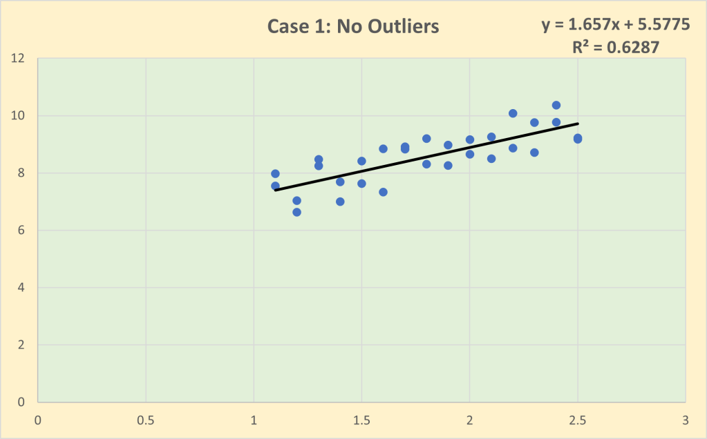
The problem with outliers is illustrated graphically below. Case 1 is the baseline with no outliers. Note that the impact (i.e. slope) coefficient of the line of best fit is 1.657 and the goodness of fit is 62.9%.
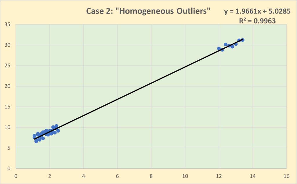
Case 2 is what I have called “homogeneous outliers” in which a group of 8 observations have been included that have unusually high values but have been generated by the same behavioural process as the baseline observations. In other words, there is structural stability across the whole dataset and hence it is legitimate to estimate a single line of best fit. Note that the inclusion of the outliers slightly increases the estimated impact coefficient to 1.966 but the goodness of fit increases substantially to 99.6%, reflecting the massive increase in the variance of the observations “explained” by the regression line.
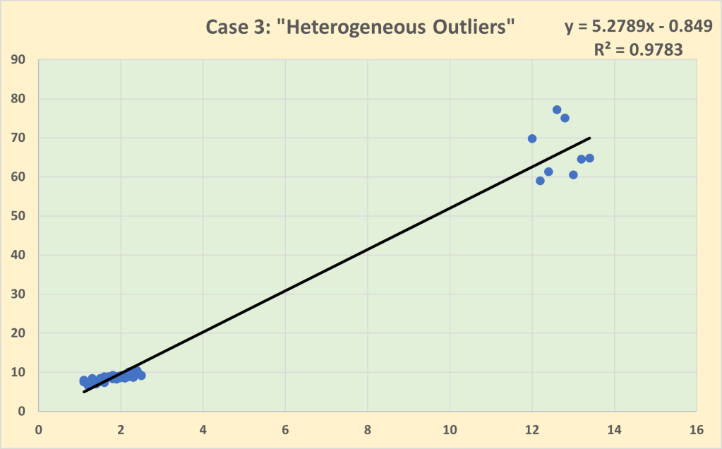
Case 3 is that of “heterogeneous outliers” in which the baseline dataset has now been expanded to include a group of 8 outliers generated by a very different behavioural process. The homogeneity assumption is no longer valid so it is inappropriate to model the dataset with a single line of best fit. If we do so, then we find that the outliers have an undue influence with the impact coefficient now estimated to be 5.279, more than double the size of the estimated impact coefficient for the baseline dataset excluding the outliers. Note that there is a slight decline in the goodness of fit to 97.8% in Case 3 compared to Case 2, partly due to the greater variability of the outliers as well as the slightly poorer fit for the baseline observations of the estimated regression line.
Of course, in this artificially generated example, it is known from the outset that the outliers have been generated by the same behavioural process as the baseline dataset in Case 2 but not in Case 3. The problem we face in real-world situations is that we do not know if we are dealing with Case 2-type outliers or Case 3-type outliers. We need to explore the dataset to determine which is more likely in any given situation.
There are a number of very simple techniques that can be used to identify possible outliers. Three of the most useful are:
- Exploratory data visualisation
- Summary statistics
- Marsh & Elliott outlier thresholds
1.Exploratory data visualisation
Histograms and scatterplots as always should be the first step in any exploratory data analysis to “eyeball” the data and get a sense of the distributional properties of the data and the pairwise relationships between all of the measured variables.
2.Summary statistics
Descriptive statistics provide a formalised summary of the distributional properties of variables. Outliers at one tail of the distribution will produce skewness that will result n a gap between the mean and median. If there are outliers in the upper tail, this will tend to inflate the mean relative to the median (and the reverse if the outliers are in the lower tail). It is also useful to compare the relative dispersion of the variables. I always include the coefficient of variation (CoV) in the reported descriptive statistics.
CoV = Standard Deviation/Mean
CoV uses the mean to standardise the standard deviation for differences in measurement scales so that the dispersion of variables can be compared on a common basis. Outliers in any particular variable will tend to increase CoV relative to other variables.
3. Marsh & Elliott outlier thresholds
Marsh & Elliott define outliers as any observation that lies more than 150% of the interquartile range beyond either the first quartile (Q1) or the third quartile (Q3).
Lower outlier threshold: Q1 – [1.5(Q3 – Q1)]
Upper outlier threshold: Q3 + [1.5(Q3 – Q1)]
I have found these thresholds to be useful rules of thumb to identify possible outliers.
Another very useful technique for identifying outliers is cluster analysis which will be the subject of a later post.
So what should you do if the exploratory data analysis indicates the possibility of outliers in your dataset? As the artificial example illustrated, outliers (just like multicollinearity) need not necessarily create a problem for modelling a dataset. The key point is that exploratory data analysis should alert you to the possibility of problems so that you are aware that you may need to take remedial actions when investigating the multivariate relationships between outcome and situational variables at the Modelling stage. It is good practice to report estimated models including and excluding the outliers in order to understand their impact on the results. If there appears to be a sizeable difference in one or more of the estimated coefficients when the outliers are included/excluded, then you should formally test for structural instability using F-tests (often called Chow tests). Testing for structural stability in both cross-sectional and longitudinal/time-series data will be discussed in more detail in a future post. Some argue to drop outliers from the dataset but personally I am loathe to discard any data which may contain useful information. Knowing the impact of the outliers on the estimated coefficients can be useful information and, indeed, it may be that further investigation into the specific conditions of the outliers could prove to be of real practical value.
The two main takeaway points are that (1) a key component of exploratory data analysis should always be checking for the possibility of outliers; and (2) if there are outliers in the dataset, ensure that you investigate their impact on the estimated models you report. You must avoid providing actionable insights that have been unduly influenced by outliers that are not representative of the actual situation with which you are dealing.
Read Other Related Posts

