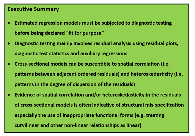
Analytical models takes the following general form:
Outcome = f(Performance, Context) + Stochastic Error
The structural model represents the systematic (or “global”) variation in the process outcome associated with the variation in the performance and context variables. The stochastic error acts as a sort of “garbage can” to capture “local” context-specific influences on process outcomes that are not generalisable in any systematic way across all the observations in the dataset. All analytical models assume that the structural model is well specified and the stochastic error is random. Diagnostic testing is the process of checking that these two assumptions hold true for any estimated analytical model.
Diagnostic testing involves the analysis of the residuals of the estimated analytical model.
Residual = Actual Outcome – Predicted Outcome
Diagnostic testing is the search for patterns in the residuals. It is a matter of interpretation as to whether any patterns in the residuals are due to structural mis-specification problems or stochastic error mis-specification problems. But structural problems must take precedence since, unless the structural model is correctly specified, the residuals will be biased estimates of the stochastic error since they will be contaminated by structural mis-specification. In this post I am focusing on structural mis-specification problems associated with cross-sectional data in which the dataset comprises observations of similar entities at the same point in time. I label this type of residual analysis as “spatial diagnostics”. I will utilise all three principal methods for detecting systematic variation in residuals: residual plots, diagnostic test statistics, and auxiliary regressions.
Data
The dataset being used to illustrate spatial diagnostics was originally extracted from the Family Expenditure Survey in January 1993. The dataset contains information on 608 households. Four variables are used – weekly household expenditure (EXPEND) is the outcome variable to be modelled by weekly household income INCOME), the number of adults in the household (ADULTS) and the age of the head of the household (AGE) which is defined as whoever is responsible for completing the survey. The model is estimated using linear regression.
Initial Model
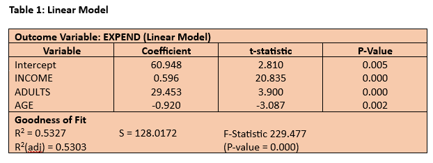
The estimated linear model is reported in Table 1 below. On the face of it, the estimated model seems satisfactory, particularly for such a simple cross-sectional model, with around 53% of the variation in weekly expenditure being explained statistically by variation in weekly income, the number of adults in the household and the age of the head of household (R2 = 0.5327). All three impact coefficients are highly significant (P-value < 0.01). The t-statistic provides a useful indicator of the relative importance of the three predictor variables since it effectively standardises the impact coefficients using their standard errors as a proxy for the units of measurement. Not surprisingly, weekly household expenditure is principally driven by weekly household income with, on average, 59.6p spent out of every additional £1 of income.

Diagnostic Tests
However, despite the satisfactory goodness of fit and high statistical significance of the impact coefficients, the linear model is not fit for purpose in respect of its spatial diagnostics. Its residuals are far from random as can be seen clearly in the two residual plots in Figures 1 and 2. Figure 1 is the scatterplot of the residuals against the outcome variable, weekly expenditure. The ideal would be a completely random scatterplot with no pattern in either the average value of the residual which should be zero (i.e. no spatial correlation) or in the degree of dispersion (known as “homoskedasticity”). In other words, the scatterplot should be centred throughout on the horizontal axis and there should also be a relatively constant vertical spread of the residual around the horizontal axis. But the residuals for the linear model are clearly trended upwards in both value (i.e. spatial correlation) and dispersion (i.e. heteroskedasticity). In most cases in my experience this sort of pattern in the residuals is caused by wrongly treating the core relationship as linear when it is better modelled as a curvilinear or some other form of non-linear relationship.

Figure 2 provides an alternative residual plot in which the residuals are ordered by their associated weekly expenditure. Effectively this plot replaces the absolute values of weekly expenditure with their rankings from lowest to highest. Again we should ideally get a random plot with no discernible pattern between adjacent residuals (i.e. no spatial correlation) and no discernible pattern in the degree of dispersion (i.e. homoskedasticity). Given the number of observations and the size of the graphic it is impossible to determine visually if there is any pattern between the adjacent residuals in most of the dataset except in the upper tail. But the degree of spatial correlation can be measured by applying the correlation coefficient to the relationship between ordered residuals and their immediate neighbour. Any correlation coefficient > |0.5| represents a large effect. In the case of the ordered residuals for the linear model of weekly household expenditure the spatial correlation coefficient is 0.605 which provides evidence of a strong relationship between adjacent ordered residuals i.e. the residuals are far from random.

So what is causing the pattern in the residuals? One way to try to answer this question is to estimate what is called an “auxiliary regression” in which regression analysis is applied to model the residuals from the original estimated regression model. One widely used form of auxiliary regression is to use the squared residuals as the outcome variable to be modelled. The results for this type of auxiliary regression applied to the residuals from the linear model of weekly household regression are reported in Table 2. The auxiliary regression overall is statistically significant (F = 7.755, P-value = 0.000). The key result is that there is a highly significant relationship between the squared residuals and weekly household income, suggesting that the next step is to focus on reformulating the income effect on household expenditure.

Revised Model and Diagnostic Tests
So diagnostic testing has suggested the strong possibility that modelling the income effect on household expenditure as a linear effect is inappropriate. What is to be done? Do we need to abandon linear regression as the modelling technique? Fortunately the answer is “not necessarily”. Although there are a number of non-linear modelling techniques, it is in most cases possible to continue using linear regression by transforming the original variables. Instead of changing the estimation method, the alternative is to transform the original variables such that there is a linear relationship between the transformed variables that is amenable to estimation by linear regression. One commonly used transformation is to introduce the square of a predictor alongside the original predictor to capture a quadratic relationship. Another common transformation is to convert the model into a loglinear form by using logarithmic transformations of the original variables. It is the latter approach that I have used as a first step in attempting to improve the structural specification of the household expenditure model. Specifically, I have replaced the original expenditure and income variables, EXPEND and INCOME, with their natural log transformations, LnEXPEND and LnINCOME, respectively. The results of the regression analysis and diagnostic testing of the new loglinear model are reported below.


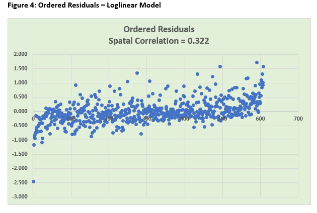
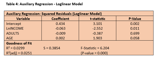
The estimated regression model is broadly similar in respect of its goodness of fit and statistical significance of the impact coefficients although, given the change in the functional form, these are not directly comparable. The impact coefficient on LnINCOME is 0.674 which represents what economists term “income elasticity” and implies that, on average, a 1% change in income is associated with a 0.67% change in expenditure in the same direction. The spatial diagnostics have improved although the residual scatterplot still shows evidence of a trend. The ordered residuals appear much more random than previously with the spatial correlation coefficient having been nearly halved and now evidence only of a medium-sized effect (> |0.3|) between adjacent residuals. The auxiliary regression is still significant overall (F = 6.204; P-value = 0.000) and, although the loglinear specification has produced a better fit for the income effect (with a lower t-statistic and increased P-value), it has had an adverse impact on the age effect (with a higher t-statistic and a P-value close to being significant at the 5% level). The conclusion – the regression model of weekly household expenditure remains “work in progress”. The next steps might be to consider extending the log transformation to the other predictors and/or introducing a quadratic age effect.
Other Related Posts
