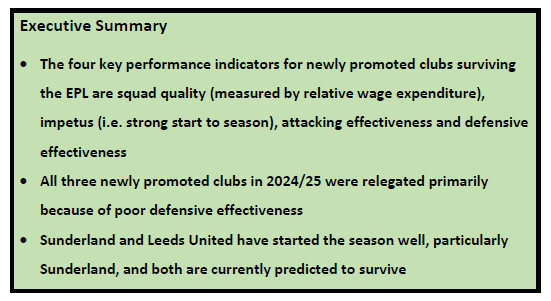
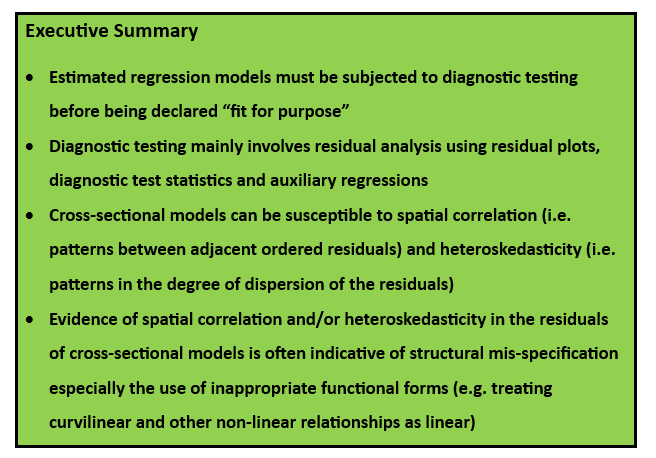
Latest Posts

Featured

The Drivers of Sporting Efficiency

Executive Summary

  • The basic production process in pro team sports is converting financial expenditure on playing talent into sporting performance
  • Any process can be summarised as Resource x Efficiency = Performance
  • Sporting efficiency is measured by the wage cost per win (i.e. the win-cost ratio)
  • Teams pursuing a “David” strategy seek high sporting performance on a limited financial budget by achieving high levels of sporting efficiency
  • Sporting efficiency can be decomposed into two components: (i) transactional efficiency i.e. maximising the quality of playing talent acquired per unit wage cost; and (ii) transformational efficiency i.e. maximising the sporting performance of a given playing squad
  • The original Moneyball story was about how the Oakland A’s used data analytics to achieve exceptional levels of transactional efficiency in recruitment
  • The “new” Moneyball story is how teams are using data analytics to maximise transformational efficiency 

All professional sports teams consist of two operations: (i) the sporting operation which produces the team’s core product, namely, on-the-field sporting performance; and (ii) the business operation tasked with monetarising the sporting performance through a variety of revenue streams, principally matchday receipts, media, sponsorship and merchandising. The basic production process in professional team sports is the conversion of financial expenditure on playing talent into sporting performance. Simply put, pro sports teams are in the business of turning wages into wins.

            Any process can be summarised  as

RESOURCE x EFFICIENCY = PERFORMANCE

In the case of pro sports teams, the resource (i.e. input) is the financial budget available to spend on playing talent. For the moment to keep things simple, let us assume initially that the resource represents wage expenditure on players. Performance is sporting performance which , again for simplicity, we will assume initially comprises competing in a league with performance measured by wins or league points. The efficiency of any process represents the rate at which input can be converted into output. Sporting efficiency is measured by the rate at which wage expenditure can be converted into wins (or league points). It is conventional to express sporting efficiency as the wage cost per win, often referred to as the win-cost ratio. In leagues with tied games and/or bonus points, sporting efficiency is best measured as the wage cost per point.

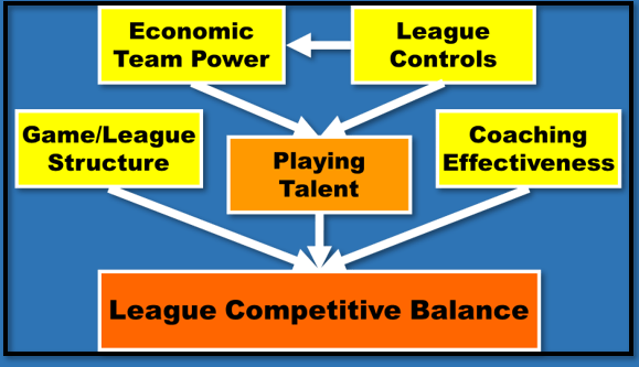
            The Resource-Efficiency relationship captures the strategic differences between teams. Typically leagues consist of a mix of big-market teams and smaller teams. The big-market teams are usually located in big metropolitan areas and have a history of sporting success. Their fanbases are large and loyal so that these teams are economically powerful, financial Goliaths in sporting terms who are able to afford large player wage budgets which gives them a strategic advantage over the smaller teams. The economically smaller teams with more limited financial budgets can only remain competitive in a financially sustainable way by developing a “David” strategy to achieve high levels of sporting efficiency. Leagues concerned about the competitive dominance of the big-market teams often attempt to restrict the resource differential between teams through measures such as (i) salary caps and other financial restrictions on player wage expenditures; (ii) revenue redistribution through centralised media and sponsorship deals; and (iii) direct controls on the player labour market including centralised player drafts.

            Sporting efficiency can be decomposed into two components: transactional efficiency and transformational efficiency. Transactional efficiency refers to the efficiency with which teams spend their player wage budget to acquire playing talent. Teams with high transactional efficiency maximise the quality of playing talent acquired per unit wage cost. Transformational efficiency refers to the efficiency with which a playing squad is trained and utilised to win sporting contests. Transformational efficiency is all about maximising the sporting performance achieved by a given playing squad. Transactional efficiency is the responsibility of the recruitment department whereas transformational efficiency is the responsibility of the coaching staff and the other sporting support staff. Transactional and transformational efficiency are interdependent. Effective recruitment is not solely about identifying high-quality players undervalued in the market. These players must be high quality in team-specific terms by which I mean, players with the qualities to be able to adapt and perform within the specific training regime and playing style of the team.

Figure 1: Decomposing Sporting Efficiency

In recent years there has been considerable focus on the use of data analytics as a  key element in the David strategy of teams seeking to maximise sport efficiency. The original Moneyball story was about how the Oakland A’s used data analytics to achieve exceptional levels of transactional efficiency in recruitment. At the core of the A’s analytics-driven recruitment strategy was their innovative use of On-Base Percentage (OBP) as a key metric to identify undervalued batters. In a study that I published in 2007, I estimated that the A’s were 59.3% more efficient than the MLB average over the period 1998-2007 which represents Billy Beane’s first nine seasons as GM. This calculation was based on the win-cost ratio after allowing for wage inflation.

            What I call the “New Moneyball” is the application of data analytics to enhance the transformational efficiency of teams. In this respect, I find it useful to think of playing talent holistically using what I call the 4 A’s – Ability (i.e. technical skills), Athleticism (i.e. physical skills), Attitude (i.e. mental skills) and Awareness (i.e. decision skills). Data analytics is contributing to all of these aspects of playing talent, augmenting the work of coaches, sport scientists, strength and conditioning trainers and sport psychologists.

            One final issue – the simplifying assumptions in the measurement of both the cost of playing talent and sporting performance need to be reviewed. As regards the cost of playing talent, there is the complication of how to treat transfer fees particularly given their importance in (association) football. One alternative is that adopted by Tomkins et al, Pay As You Play (GPRF Publishing, 2010) who provided a detailed analysis of what they called “the price of success” in the English Premier League (EPL), 1992 – 2010, using their Transfer Price Index. Their efficiency measure was the transfer cost per league point using the inflation-adjusted transfer value of the playing squad. Another approach is what I would call “the full-cost method” in which acquisition costs are included as well as wage costs. The simplest version of this method is to combine the annual amortisation charge on transfer fees paid with annual wages and salaries. My own preference is to use the wages-only method in analysing what I would call “operating-cost sporting efficiency” and to separately analyse the ”capital-cost sporting efficiency” of transfer fees paid and received.

            As regards the measurement of sporting performance, the principal problem again arises primarily in football when the top teams compete in two elite tournaments – their own domestic league and an international tournament. For example, top English teams compete in both the EPL and the UEFA Champions League. Their sporting efficiency should be assessed in terms of their performance in both tournaments. But trying to a create a composite measure of sporting performance in multiple tournaments is difficult and aways open to the charge of arbitrariness. So, just as in the case of the measurement of player costs, I advocate separability i.e. analyse the efficiency of sporting performance in different tournaments separately. Ultimately it comes down to making meaningful comparisons using metrics that are transparent and measured consistently to ensure that we are comparing like with like as much as possible. So, for example, it is much more informative to compare the wage cost per point of the EPL teams competing in the UEFA Champions League with each other and then separately compare the wage cost per point of the other EPL teams.

Other Related Posts

Diagnostic Testing Part 2: Spatial Diagnostics

Analytical models takes the following general form:

Outcome = f(Performance, Context) + Stochastic Error

The structural model represents the systematic (or “global”) variation in the process outcome associated with the variation in the performance and context variables. The stochastic error acts as a sort of “garbage can” to capture “local” context-specific influences on process outcomes that are not generalisable in any systematic way across all the observations in the dataset. All analytical models assume that the structural model is well specified and the stochastic error is random. Diagnostic testing is the process of checking that these two assumptions hold true for any estimated analytical model.

Diagnostic testing involves the analysis of the residuals of the estimated analytical model.

Residual = Actual Outcome – Predicted Outcome

Diagnostic testing is the search for patterns in the residuals. It is a matter of interpretation as to whether any patterns in the residuals are due to structural mis-specification problems or stochastic error mis-specification problems. But structural problems must take precedence since, unless the structural model is correctly specified, the residuals will be biased estimates of the stochastic error since they will be contaminated by structural mis-specification. In this post I am focusing on structural mis-specification problems associated with cross-sectional data in which the dataset comprises observations of similar entities at the same point in time. I label this type of residual analysis as “spatial diagnostics”. I will utilise all three principal  methods for detecting systematic variation in residuals: residual plots, diagnostic test statistics, and auxiliary regressions.

Data

The dataset being used to illustrate spatial diagnostics was originally extracted from the Family Expenditure Survey in January 1993. The dataset contains information on 608 households. Four variables are used – weekly household expenditure (EXPEND) is the outcome variable to be modelled by weekly household income INCOME), the number of adults in the household (ADULTS) and the age of the head of the household (AGE) which is defined as whoever is responsible for completing the survey. The model is estimated using linear regression.

Initial Model

The estimated linear model is reported in Table 1 below. On the face of it, the estimated model seems satisfactory, particularly for such a simple cross-sectional model, with around 53% of the variation in weekly expenditure being explained statistically by variation in weekly income, the number of adults in the household and the age of the head of household (R2 = 0.5327). All three impact coefficients are highly significant (P-value < 0.01). The t-statistic provides a useful indicator of the relative importance of the three predictor variables since it effectively standardises the impact coefficients using their standard errors as a proxy for the units of measurement. Not surprisingly, weekly household expenditure is principally driven by weekly household income with, on average, 59.6p spent out of every additional £1 of income.

Diagnostic Tests

However, despite the satisfactory goodness of fit and high statistical significance of the impact coefficients, the linear model is not fit for purpose in respect of its spatial diagnostics. Its residuals are far from random as can be seen clearly in the two residual plots in Figures 1 and 2. Figure 1 is the scatterplot of the residuals against the outcome variable, weekly expenditure. The ideal would be a completely random scatterplot with no pattern in either the average value of the residual which should be zero (i.e. no spatial correlation) or in the degree of dispersion (known as “homoskedasticity”). In other words, the scatterplot should be centred throughout on the horizontal axis and there should also be a relatively constant vertical spread of the residual around the horizontal axis. But the residuals for the linear model are clearly trended upwards in both value (i.e. spatial correlation) and dispersion (i.e. heteroskedasticity). In most cases in my experience this sort of pattern in the residuals is caused by wrongly treating the core relationship as linear when it is better modelled as a curvilinear or some other form of non-linear relationship.

            Figure 2 provides an alternative residual plot in which the residuals are ordered by their associated weekly expenditure. Effectively this plot replaces the absolute values of weekly expenditure with their rankings from lowest to highest. Again we should ideally get a random plot with no discernible pattern between adjacent residuals (i.e. no spatial correlation) and no discernible pattern in the degree of dispersion (i.e. homoskedasticity). Given the number of observations and the size of the graphic it is impossible to determine visually if there is any pattern between the adjacent residuals in most of the dataset except in the upper tail. But the degree of spatial correlation can be measured by applying the correlation coefficient to the relationship between ordered residuals and their immediate neighbour. Any correlation coefficient > |0.5| represents a large effect. In the case of the ordered residuals for the linear model of weekly household expenditure the spatial correlation coefficient is 0.605 which provides evidence of a strong relationship between adjacent ordered residuals i.e. the residuals are far from random.

            So what is causing the pattern in the residuals? One way to try to answer this question is to estimate what is called an “auxiliary regression” in which regression analysis is applied to model the residuals from the original estimated regression model. One widely used form of auxiliary regression is to use the squared residuals as the outcome variable to be modelled. The results for this type of auxiliary regression applied to the residuals from the linear model of weekly household regression are reported in Table 2. The auxiliary regression overall is statistically significant (F = 7.755, P-value = 0.000). The key result is that there is a highly significant relationship between the squared residuals and weekly household income, suggesting that the next step is to focus on reformulating the income effect on household expenditure.

Revised Model and Diagnostic Tests

So diagnostic testing has suggested the strong possibility that modelling the income effect on household expenditure as a linear effect is inappropriate. What is to be done? Do we need to abandon linear regression as the modelling technique? Fortunately the answer is “not necessarily”. Although there are a number of non-linear modelling techniques, it is in most cases possible to continue using linear regression by transforming the original variables. Instead of changing the estimation method, the alternative is to transform the original variables such that there is a linear relationship between the transformed variables that is amenable to estimation by linear regression. One commonly used transformation is to introduce the square of a predictor alongside the original predictor to capture a quadratic relationship. Another common transformation is to convert the model into a loglinear form by using logarithmic transformations of the original variables. It is the latter approach that I have used as a first step in attempting to improve the structural specification of the household expenditure model. Specifically, I have replaced the original expenditure and income variables, EXPEND and INCOME, with their natural log transformations, LnEXPEND and LnINCOME, respectively. The results of the regression analysis and diagnostic testing of the new loglinear model are reported below.

The estimated regression model is broadly similar in respect of its goodness of fit and statistical significance of the impact coefficients although, given the change in the functional form, these are not directly comparable. The impact coefficient on LnINCOME is 0.674 which represents what economists term “income elasticity” and implies that, on average, a 1% change in income is associated with a 0.67% change in expenditure in the same direction. The spatial diagnostics have improved although the residual scatterplot still shows evidence of a trend. The ordered residuals appear much more random than previously with the spatial correlation coefficient having been nearly halved and now evidence only of a medium-sized effect (> |0.3|) between adjacent residuals. The auxiliary regression is still significant overall (F = 6.204; P-value = 0.000) and, although the loglinear specification has produced a better fit for the income effect (with a lower t-statistic and increased P-value), it has had an adverse impact on the age effect (with a higher t-statistic and a P-value close to being significant at the 5% level). The conclusion – the regression model of weekly household expenditure remains “work in progress”. The next steps might be to consider extending the log transformation to the other predictors and/or introducing a quadratic age effect.

Other Related Posts

Diagnostic Testing Part 1: Why Is It So Important?

Competitive Balance Part 3: North American Major Leagues

As discussed in the two previous posts on competitive balance, there is no agreed single definition of competitive balance beyond a general statement that a competitively balanced league is characterised by all teams having a relatively equal chance of winning individual games and the league championship. The lack of agreement on a specific definition of competitive balance combined with the wide variety of league structures and the statistical problems of inferring ex ante (i.e. pre-event) success probabilities from ex post (i.e. actual) league outcomes has led to a multiplicity of competitive balance metrics. Morten Kringstad and I have argued in several published journal articles and book chapters that it is useful to categorise competitive balance metrics as either measures of win dispersion or performance persistence. Win dispersion measures the dispersion in league performance across teams in a particular season. Performance persistence measures the degree to which the league performance of individual teams is replicated across seasons – do teams tend to finish in the same league position in consecutive seasons? These are two quite different aspects of competitive balance and multiple metrics have been proposed for both. However, when it comes to discussions as to what leagues should do, if anything, to maintain or improve of competitive balance, there is a general (often implicit) presumption that all competitive balance metrics tend to move in the same direction. Morten and I have sought to discover if this is indeed the case. And, as reported in my previous post on the subject, the evidence from European football is quite mixed and, at the very least, casts doubt on the general presumption that there is a strong positive relationship between win dispersion and persistence. Indeed, we found that in the period 2008 – 2017 win dispersion and performance persistence tended to move in opposite directions in the English Premier League.

            In this post, I am going to discuss the evidence from a study on win dispersion and performance persistence in the four North American Major Leagues (NAMLs) that Morten and I published recently in Sport, Business, Management: An International Journal (vol 13 no. 5, 2023). Our dataset covered the four NAMLs – MLB (baseball), NFL (American football), NBA (basketball) and NHL (ice hockey) – seven different competitive balance metrics, and 60 seasons, 1960 – 2019 (thereby avoiding the impact of the Covid pandemic). In this post I am only focusing on the ASD* measure of win dispersion, the SRCC measure of performance persistence, and the correlation between these measures to test whether or not win dispersion and performance persistence move together in the same direction. I have reported these three measures as 10-year averages in order to identify possible trends over time. It is agreed that the ASD* metric provides better comparability of win dispersion between leagues with very different lengths of game schedules in the regular season. At one extreme the MLB has a 162-game schedule whereas for most of the period the NFL had a 16-game regular season schedule (recently increased to 17 games). The ASD* uses the actual standard deviation of team win percentages relative to the theoretical standard deviation of a perfectly dominated league with the same number of teams and games in which every team loses against the teams ranked above it so the top team wins every game, the second best team only loses against the top team, the 3rd-placed team only loses against the top two and so on. (Formally, this is called a “cascade” distribution.) The SRCC measure of performance persistence is just the Spearman rank correlation coefficient of league standings in two consecutive seasons.

            One important contextual change in most leagues since the 1960s has been the move away from a very restricted player labour market in which a player’s current team had priority in retaining a player. Instead player labour markets have become a very competitive auction-type market in which players have the right to move to another team at the end of their current contract (what is known as “free agency”). The NAML’s led the way in pro team sports in introducing some form of free agency in the 1970s/80s. European leagues lagged behind until the Bosman ruling in 1995 which effectively created free agency by abolishing transfer fees for out-of-contract players. So in some ways it should be expected that the general trend in the NAMLs has been towards greater competitive imbalance as the big-market teams have taken advantage of free agency to acquire the best players. However, there has been another general tendency with leagues becoming much more interventionist by introducing regulatory mechanisms especially salary caps which, in part, has been motivated by an attempt to offset the potential negative effect on competitive balance of free agency. Which effect has been stronger? Let’s look at the numbers.

            Table 1 below reports the 10-year averages for win dispersion for the four NAMLs. Broadly speaking, the pattern in win dispersion in the NAMLs over the last 60 years has been for win dispersion to decrease from the 1960s though to the 1990s (i.e. improved competitive balance) but for win dispersion to increase since the 1990s (i.e. reduced competitive balance). Both the MLB and NFL follow this pattern, suggesting that the league intervention effect may have initially dominated the free agency effect but in recent years the resource-richer teams may have adapted to the more regulated environment and found other ways to exert their financial advantage (while remaining compliant with league regulations) such as higher expenditures on technology and data analytics. I used to argue that the Oakland A’s and the Moneyball phenomenon is an example of data analytics being used as a “David” strategy for resource-poorer teams to compete more effectively. And it is true that in the early days of sports analytics it was often the resource-poorer teams that led the way in operationalising data analytics as a source of competitive advantage. But these days most teams recognise the potential gains from analytics and some very resource-rich teams are investing heavily in data analytics.

            The trends in win dispersion are much less clear in both the NBA and NHL. There has been some underlying trend from the 1960s onwards for competitive balance to worsen in the NBA as win dispersion has increased. In contrast, the NHL has tended to experience an improvement in competitive balance with lower win dispersion since the turn of the century.

            When win dispersion across the four NAMLs are compared, there is a rather surprising result that the NFL has the highest degree of win dispersion over the whole period (i.e. low competitive balance) whereas the MLB has the lowest win dispersion (i.e. high competitive balance) with the NBA and NHL in the mid-range. I say surprising since conventional wisdom is that NFL has been one of the most proactive leagues in trying to maintain a high level of competitive balance whereas traditionally the MLB has been much less interventionist. The problem in making comparisons across leagues especially in different sports is the “apples-and-oranges” problem – trying to compare like with like. As highlighted earlier, there are massive differences between the NAMLs in the length of regular-season game schedules. I am more inclined to the view that the difference in win dispersion between the NAMLs is more a reflection of the difficulties in constructing a metric that properly controls for the length of game schedules, that is, it is more a measurement problem than a “true” reflection of differences in competitive balance.

            The argument that win dispersion metrics can pick up trends within leagues but is less reliable for comparisons across leagues is reinforced by the results for performance persistence reported below in Table 2. Performance persistence measures the degree to which the final standings of teams are replicated in consecutive seasons. The length of game schedule has a much more indirect effect on performance persistence so that comparisons across leagues should be more reliable. And, indeed, we find that from the 1980s onwards the NFL has had the lowest degree of performance persistence which fits with the conventional view that the NFL has been the most proactive league in maintaining a high degree of competitive balance. Winning NFL teams face a number of “penalties” in the next season – tougher game schedules, lower-ranked draft picks and the constraints imposed by the salary cap in retaining free agents who have increased in value by virtue of their on-the-field success. It is more and more difficult for NFL teams to become “dynasty” teams which makes the Belichick-Brady era at the New England Patriots and, most recently, the success of the Kansas City Chiefs so remarkable.

            As well as the NFL, the other NAML that has managed to reduce the degree of performance persistence is the NHL which had the highest degree of performance persistence in the 1960s and 1970s but now ranks second best behind the NFL. The MLB experienced reduced performance persistence in the 1980s and 1990s ( and had, on average, lower performance persistence than the NFL in the 1990s) but that downward trend has been reversed in the last two decades. The one major league that has had no discernible trend in performance persistence over the last 60 years and has the highest degree of performance persistence is the NBA despite instituting a salary cap albeit a rather “soft” cap with a number of exemptions. The high performance persistence of basketball teams is inherent in the very structure of the game. With only five players on court for a team at any point in time, basketball is much more susceptible to the “Michael Jordan” (i.e. “super-superstar”) effect and the soft salary cap makes it easier to retain these super-superstars.

            The final set of results reported in Table 3 show how the relationship between win dispersion and performance persistence has varied over time and between leagues. One of the main motivations for this research is to determine whether or not the general presumption of a strong positive dispersion-persistence relationship is empirically valid. The evidence is mixed. There are only eight instances of a strong positive dispersion-persistence relationship (r > 0.5) out of a possible 24 which is hardly overwhelming evidence in favour of the general presumption. If medium-sized effects are included (0.3 < r < 0.5) then only half of the reported results provide support for the general presumption of a positive relationship with three strong/medium negative results and nine showing only small/negligible effects. There is one instance of a strong negative dispersion-persistence relationship in the NHL in 2010-19 indicating that reductions in performance persistence were associated with increases in win dispersion.

Competitive balance in the NAMLs has been much researched over the last 30 years. The results of our study are broadly in line with previous results but highlight that any conclusions are likely to be time-dependent and metric-dependent. The most definitive results are those on performance persistence which show a general tendency in both the NFL and NHL for improved competitive balance despite the advent of free agency. There is also clear evidence of  continuing high levels of performance persistence in the NBA, likely to be due to the super-superstar effect inherent in the game structure of basketball. As for the general presumption that win dispersion and performance persistence tend to move together in the same direction, there is no overwhelming support that they do so in most cases. The practical implication is that leagues need to be clearer on which aspect of competitive balance is most important in driving uncertainty of outcome and spectator/viewer interest. Leagues must also recognise that the structures of their sports may limit the extent to which competitive balance can be regulated. Basketball is always likely to more susceptible to super-superstar effects that can lead to high levels of performance persistence. And leagues with short game schedules may always tend to have higher levels of win dispersion since there is more limited opportunity for winning or losing streaks to even themselves out – what statisticians call the “regression-to-the-mean” effect.

Other Related Posts

Competitive Balance Part 1: What Are The Issues?

Competitive Balance Part 2: European Football

Note: The results reported in this post are published in B. Gerrard and M. Kringstad, ‘Dispersion and persistence in the competitive balance of North American Major Leagues 1960 – 2019‘, Sport, Business, Management: An International Journal, vol. 13 no. 5 (2023), pp. 640-662.

Economic Forecasting: What Is Going On?

The Times ran an editorial last Saturday (‘Predictable Mistakes’, Times, 3 Feb 2024) that was highly critical of economic forecasting particularly in the UK, pointing out that ‘among leading economies, British forecasters have distinguished themselves as the least prescient of the lot.’ A harsh assessment indeed and one with very serious consequences for all of us since, as the editorial went on to say, ‘bad modelling lays the ground for bad policymaking affecting investment strategy and monetary policy.’

            The Times editorial follows two recent columns in the Sunday Times which were also highly critical of economic forecasting. Dominic Lawson (‘Forecasts have one tiny flaw: they’re useless’, Sunday Times, 31 Dec 2023) compared economic forecasters to the augurs in Ancient Rome, a sort of priesthood distinguished by their supposed skills in predicting an uncertain future based on natural signs such as the behaviour of birds to determine whether the gods approved or disapproved of a proposed course of action. For “natural signs” read “econometrics”, but otherwise there is little difference in mindset – an overwhelming confidence, bordering on arrogance, in their superiority to the rest of us when it comes to transcending uncertainty.

              Dominic Lawson, who is the son of Nigel Lawson, the former Chancellor of the Exchequer, approvingly quoted his late father’s very perceptive comment on the fundamental problem with economic forecasting and economics in general being the illusion that because economic outcomes can be quantified, economic behaviour can be reduced to a set of mathematical equations. But, as Dominic Lawson argues, quantifiability does not mitigate the uncertainty inherent in economic behaviour. Economics is not physics; it deals with the irrationalities of economic behaviour not the behaviour of things that follow the laws of physics. And matters are made worse by the poor quality of much economic data, so much so that economic forecasters (and, hence, policymakers) are essentially flying blind. Lawson concludes his column with the rather damning comment that the time and money spent on forecasting human behaviour is a ‘monument to gullibility’. It reminds me of Deirdre McCloskey’s view that economics and econometrics are at times no more than the proverbial “snake oil”, sold by their purveyors as a cure-all but with little in the way of substantive evidence to support the marketing claims.

            Economists flying blind is the concern of Irwin Stelzer in his column, ‘Forecasting in the age of uncertainty’ (Sunday Times, 14 Jan 2024). Stelzer highlights the uncertainties in supply chains and how the interdependencies are transforming local and regional problems into global problems. It is a “butterfly effect” on a grand scale. Stelzer reminds us of the importance of Knight and Keynes as two economists who understood the difference between risk and uncertainty, and, crucially, recognised that investors fear uncertainty, not risk.

            I am reminded of a recent discussion with a senior economist of many years standing on the need for economics to embrace data analytics more thoroughly. In particular, as I have argued in recent posts, data analytics is data analysis for practical purpose and the necessary mindset for practical purpose demands a recognition of the importance of context. Although there are important differences between the approaches of Knight and Keynes (and I largely follow Keynes’s approach), both rejected the notion that uncertainty could be reduced to a well-defined probability distribution for a random process with a known, stable structure akin to the roulette wheel. The senior economist, who I would consider to be a radical economist strongly influenced by the ideas of Marx rather than modern mainstream economic theory, was very dismissive of my proposition that economics needs more data analytics. His response was that what economics needs is more sophisticated econometrics, not data analytics. Perhaps I should not have been surprised that a Marxist economist would believe in the predictability of economic forces. I suspect that Bernanke’s report on the forecasting capabilities of the Bank of England will reach a similar conclusion and argue for more sophisticated econometrics as the cure-all. But greater sophistication in econometric methods will not generate greater forecasting accuracy. Ultimately if there is no fundamental change in the mindset of economists and economic forecasters as regards the nature of uncertainty, there will be no change in the practical value of economic forecasts and policy advice. It is these issues that I intend to investigate in more detail in the coming weeks in a planned series of posts entitled ‘Risk, Probability and Uncertainty’.

Other Related Posts

Analytics and Context

Putting Data in Context

Competitive Balance Part 2: European Football

As discussed in the previous post, ‘Competitive Balance Part 1: What are the Issues?’ (24th Jan 2024), competitive balance remains an elusive concept in many ways. There is considerable disagreement over the definition and measurement of competitive balance which has generated multiple metrics. In addition, the variety of real-world nuances in the structure of sporting tournaments across different sports and different countries has exacerbated the problem as refinements to existing metrics are proposed to improve comparability across sports and countries.

Morten Kringstad and I have attempted to bring some order to the chaos by arguing that competitive balance metrics can be categorised by their timeframe and scope. In particular, as regards timeframe, competitive balance metrics either focus on the distribution of sporting outcomes of participants within a single season (i.e. win dispersion) or the degree to which to which participants replicate their level of sporting performance across seasons (i.e. performance persistence). Competitive balance metrics also differ in respect to their scope, either including all of the participants (i.e. whole league) or a subset of the strongest/weakest performers (i.e. tail outcomes).

The practical problem created by the multiplicity of competitive balance metrics is identifying which metrics should be used by league authorities in determining whether or not intervention is required to improve competitive balance. There is no general definitive empirical evidence on which aspects of competitive balance impact on gate attendances and TV viewing. There seems to be an implicit assumption that the competitive balance metrics tend to move together in the same direction, so that interventions such as centralised revenue distribution and salary caps would be expected to improve both win dispersion and performance persistence. Is this assumption valid? This is the question that Morten and I investigated in an exploratory study published in 2022 on competitive balance in European football.

Competitive Balance in European Football Leagues (EFLs)

The dataset compiled by Morten and I covers the 18 best attended, top tier domestic leagues in European football. We grouped the leagues into three groups – the Big Five (England, France, Germany, Italy and Spain), medium-sized leagues (including the Netherlands and Scotland) and the smaller–sized leagues (including Denmark and Norway). We used final league positions for ten seasons from 2008 to 2017. In the published study we reported seven alternative competitive balance metrics but found that the four win dispersion metrics were highly correlated with each other but much less so with the performance persistence metric which supports our contention of differentiating between these two types of metric. Some of the key results are reported in Table 1 below.

Table 1: Competitive Balance in European Football Leagues, 2008 – 2017

The English Premier League (EPL) stands out as the least competitively balanced of the Big Five leagues with the highest 10-year average for both win dispersion and performance dispersion. The Spanish La Liga has similar levels of competitive dominance as the EPL. In contrast, the German Bundesliga and the French Ligue 1 are the most competitively balanced. The Bundesliga has the lowest 10-year average for performance persistence across all teams. But the Bundesliga has the highest championship concentration in that period due to the dominance of Bayern Munich who won the league seven out of ten of those seasons. It is also noticeable that smaller EFLs tend to be more competitively balanced in win dispersion, performance persistence and championship concentration compared to the Big Five and the medium-sized leagues.

As regards the dispersion-performance relationship, across all 18 leagues there is a general tendency for a small positive relationship between win dispersion and performance persistence. But the dispersion-persistence relationship is highly variable across leagues especially in the Big Five. In the Spanish La Liga, which is one of the least competitively balanced leagues in our sample due to the dominance of the two global “super” teams – Real Madrid and Barcelona, there is a strong positive relationship between win dispersion and performance persistence. On the other hand, the German Bundesliga which, as highlighted above, is one of the most competitively balanced leagues despite the dominance of Bayern Munich, has a negligible dispersion-persistence relationship. The most surprising result is that for the EPL which has a strong negative relationship between win dispersion and performance persistence. The Juliper Pro League in Belgium and the Dutch Eredivisie also display a similar strong negative dispersion-persistence relationship during these ten seasons. As sporting performance becomes more dispersed across teams within a season in these three leagues, there is a tendency for sporting performance of teams to become less persistent across seasons. Perhaps this strong negative dispersion-persistence relationship is the part of the explanation of the paradox (at least in the eyes of sports economists) that the EPL is one of the least competitively balanced football leagues but remains the most commercially successful football league in the world.

What could be causing the win dispersion and performance persistence to be strongly negatively related in the EPL in defiance of the usual assumption that all competitive balance metrics tend to move together in the same direction? In our published study Morten and I develop a simple theoretical model that shows a negative dispersion-persistence relationship is more likely when there are strong persistence effects amongst the smaller teams. We suggest that the continuing growth of the value of the EPL’s media rights is putting the smaller teams in a particularly advantageous position vis-à-vis newly promoted teams and increasing the likelihood of incumbent teams avoiding relegation. And, on the other side of the coin, there is a greater likelihood of newly promoted teams becoming yo-yo teams, bouncing between the EPL and the Football League Championship.

Other Related Posts

Competitive Balance Part 1: What Are The Issues?

Financial Determinism and the Shooting-Star Phenomenon in the English Premier League

Note: The results reported in this post are published in B. Gerrard and M. Kringstad, ‘The multi-dimensionality of competitive balance: evidence from European football’, Sport, Business, Management: An International Journal, vol. 12 no. 4 (2022), pp. 382-402.

Diagnostic Testing Part 1: Why Is It So Important?

Analytical models are a simplified, purpose-led, data-based representation of a real-world problem situation. In terms of the categorisation of data proposed in the previous post, “Putting Data in Context” (24th Jan 2024), analytical models typical take the form of a multivariate relationship between the process outcome variable and a set of performance and context (i.e. predictor) variables.

Outcome = f(Performance, Context)

In evaluating the estimated models derived from a particular dataset, there are three general criteria to be considered:

  • Specification criterion: is the model as simple as possible but still comprehensive in its inclusion of all relevant variables?
  • Usability criterion: is the model fit for purpose?
  • Diagnostic testing criterion: does the model use the available data effectively?

These criteria are applicable to all estimated analytical models but the specific focus and empirical examples in this series of posts will be linear regression models.

Specification Criterion

Analytical models should only include as predictors the relevant performance and context variables that influence the (target) outcome variable. To keep the model as simple as possible, irrelevant variables with no predictive power should be excluded. In the case of linear regression models the adjusted R2 (i.e. adjusted for the number of variables and observations) is the most useful statistic for comparing the goodness of fit across linear regression models with different numbers of predictors. Maximising the adjusted R2 is equivalent to minimising the standard error of the regression and yields the model specification rule of retaining all predictors with (absolute) t-statistics > 1.

Usability Criterion

The purpose of an analytical model is to provide an evidential basis for developing an intervention strategy to improve process outcomes. There are three general requirements for a usable analytical model:

  • All systematic influences on process outcomes are included
  • Model goodness of fit is maximised
  • One or more predictor variables are controllable, that is, (i) causally linked to the process outcome; (ii) a potential target for managerial intervention; and (iii) with a sufficiently large effect size

Diagnostic Testing Criterion

A linear regression model takes the following general form:

Outcome = f(Performance, Context) + Stochastic Error

There are two components: (i) the structural model, f(.), that seeks to capture the systematic variation in the process outcome associated with the variation in the performance and context variables; and (ii) the stochastic error that represents the non-systematic variation in the process outcome. The stochastic error captures the myriad of “local” context-specific influences that impact on the individual observations but whose effects are not generalisable in any systematic way across all the observations in the dataset.

            Regression analysis, like all analytical models, assumes that (i) the structural model is well specified; and (ii) the stochastic error is random (which, in formal statistical terms, requires that the errors are identically and independently distributed). Diagnostic testing is the process of checking that these two assumptions hold true for any estimated analytical model. To use the signal-noise analogy from physics, data analytics can be seen as a signal-extraction process in which the objective is to separate the systematic information (i.e. signal) from the non-systematic information (i.e. noise). Diagnostic testing involves ensuring that all of the signal has been extracted and that the remaining information is random noise.

A Checklist of Possible Diagnostic Problems

There are three broad types of diagnostic problems:

  • Structural problems: these are potential mis-specification problems with the structural component of the analytical model and include wrong functional form, missing relevant variables, incorrect dynamics in time-series models, and structural instability (i.e. the estimated parameters are unstable across subsets of the data)
  • Stochastic error problems: the stochastic error is not well behaved and is non-independently and/or non-identically distributed
  • Informational problems: the information structure of the dataset is characterised by heterogeneity (i.e. outliers and/or clusters) and/or communality

Informational problems should be identified and resolved during the exploratory data analysis before estimating the analytical model. Diagnostic testing focuses on structural and stochastic error problems as part of the evaluation of estimated models. Within the diagnostic testing process, it is strongly recommended that priority is given to structural problems. Ultimately, as discussed below, diagnostic testing involves the analysis of the residuals of the estimated analytical model. Diagnostic testing is the search for patterns in the residuals. It is a matter of interpretation as to whether any patterns in the residuals are due to structural problems or stochastic error problems. But the solutions are quite different. Structural problems require that the structural component of the analytical model is revised whereas stochastic error problems require a different estimation method to be used. However, the residuals can only be “unbiased” estimates of the stochastic error if and only if the structural component is well specified. It comes down to mindset. If you have a “Master of the Universe” mindset and believe that the analytical model is well specified, then, from that perspective, any patterns in the residuals are a stochastic error problem requiring the use of more sophisticated estimation techniques. This is the traditional approach in econometrics by those wedded to the belief in the infallibility of mainstream economic theory and confident that theory-based models are well specified. In contrast, practitioners, if they are to be effective in achieving better outcomes, require a much greater degree of humility in the face of an uncertain world, recognising that analytical models are always fallible. Interpreting patterns in residuals as evidence of structural mis-specification is, in my experience, much more likely to lead to better, fit-for-purpose models.  

Diagnostic Testing as Residual Analysis  

Diagnostic testing largely involves the analysis of the residuals of the estimated analytical model.

Residual = Actual Outcome – Predicted Outcome

Essentially diagnostic testing is the search for patterns in the residuals. The most common types of patterns in residuals when ordered by size or time are correlations between successive residuals (i.e. spatial or serial correlation) and changes in their degree of dispersion  (known as “heteroskedasticity”). There are three principal methods for detecting systematic variation in residuals:

  • Residual plots – visualisations of the bivariate relationships between the residuals and the outcome and predictor variables
  • Diagnostic test statistics – formal hypothesis testing of the existence of systematic variation in the residuals
  • Auxiliary regressions – the estimation of supplementary regression models in which  as the outcome variable is the original (or transformed) residuals from the initial regression model

In subsequent posts I will review the use of residual analysis in both cross-sectional models (Part 2) and time-series models (Part 3). I will also consider the overfitting problem (Part 4) and structural instability (Part 5).

Other Related Posts

Putting Data in Context

Competitive Balance Part 1: What Are The Issues?

The importance of competitive balance and uncertainty of outcome for professional sports leagues is axiomatic not only in academia but also within the sports industry and the media in general. But what is competitive balance? There are a multitude of definitions and metrics. Competitive balance clearly means different things to different people. Its importance is also problematic. The English Premier League (EPL) is often cited as an example of a competitively dominated league but its gate attendances and TV ratings continue to grow, as does the value of its domestic and international media rights.

            I have long held an interest in competitive balance both as a sports economist and as a sports fan. I have presented at various academic and industry conferences and workshops on the subject over the years as well as publishing journal articles and book chapters. Much of my research on competitive balance has been in collaboration with Morten Kringstad, a Norwegian sports economist who completed a doctoral dissertation on competitive balance at Leeds University Business School

            In this post I want to discuss competitive balance in terms of four issues – definition, significance, measurement and implications. In two subsequent posts I will present empirical evidence on competitive balance in both European football and the North American major leagues that Morten and I have published in recent journal articles.

Definition

What is competitive balance? In the most general sense, competitive balance is the distribution across teams of the probability of sporting success in a league. (Although my focus is primarily with competitive balance in professional teams sports in which teams compete in a league-structured tournament, competitive balance can apply to both individual and team sports and to both league and elimination tournaments.) Perfect competitive balance implies that all teams in a league have an equal probability of sporting success. This, in turn, would require an equal distribution of playing and coaching talent across all teams. Competitive dominance (i.e. competitive imbalance) implies that a small number of teams in a league have high probabilities of sporting success with all the other teams having close to zero probability of sporting success.

Significance

Why is competitive balance important? Sports economists have long argued that uncertainty of outcome is a necessary requirement for the financial viability of professional sports leagues. Sporting contests are unscripted drama in which there is no need for the audience to suspend their belief to create uncertainty over the outcome. But teams vary in their economic power as a matter of history and geography. Teams located in large metropolitan areas have a larger potential local fanbase. Fans from outside the team’s local catchment area are often attracted by a team’s current success. The bigger a team’s fanbase, the bigger its potential economic power to monetise its sporting operations through gate receipts, corporate hospitality, merchandising, sponsorship and media rights. There is also the possibility of non-indigenous economic power through the acquisition of the team by a wealthy ownership. The constant threat is a league may become competitively dominated by a small group of very economically powerful teams, possibly just one “super” team, so that there is no longer any real uncertainty of outcome leading to a loss of general engagement with the league and the consequent decline in revenues.

Measurement

How is competitive balance measured? Competitive balance is an ex ante concept in the sense that it refers to expected sporting outcomes. Competitive balance is most appropriately measured by betting odds or the actual distribution of playing and coaching resources (or the financial resources available to teams to spend on their sporting operations). Within the academic literature, the empirical focus has typically been on ex post competitive outcomes i.e. the distribution of actual sporing performance across teams.

            As I indicated in my introductory remarks, one of the main problems in the research on competitive balance is the large number of alternative metrics. One of main themes of my research, particularly my collaboration with Morten Kringstad, has been to construct a classification system to bring some order to the chaos of the multiple competitive balance metrics. Essentially competitive balance metrics can be classified in terms of two dimensions – timeframe and scope. As regards the timeframe, competitive balance metrics can be grouped into those focused on competitive balance in a single season and those that focus on multiple seasons. Single-season metrics are termed “win dispersion” and seek to measure the distribution of sporting outcomes across teams in one league season. The original formulation of this metric is the relative standard deviation (RSD) which measures the actual standard deviation of team win percentages as a ratio of the standard deviation for an ideal league of the same size in which every team has a 50-50 chance of winning every game (statistically this ideal league is modelled as a binomial distribution with match outcomes treated as equivalent to a fair coin toss). Multiple-season measures are termed “performance persistence” and measure the extent to which teams replicate the same level of performance across seasons. One widely used measure of performance persistence is the rank correlation of league positions of teams in successive seasons.

Win dispersion and performance persistence represent different aspects of competitive balance – is a league characterised in each season by teams being closely grouped together with similar win-loss records (i.e. low win dispersion)? do the same teams tend to finish towards the top/middle/bottom of the league every season (i.e. high performance persistence)? Win dispersion and performance persistence are not the same thing and it is not clear which is more important in driving gate attendances and TV ratings. And win dispersion and performance persistence need not necessarily move together over time. (The dispersion-persistence relationship is a particular focus of the empirical evidence to be presented in subsequent posts on competitive balance.)

            The scope dimension refers to whether the competitive balance metrics are calculated for the whole league using the sporting outcomes of all teams (whole-league metrics) or are focused on just the top and/or bottom of the leagues (tail-outcome metrics). One widely reported tail-outcome metric is the concentration of league championship titles. Other tail-outcome metrics include those measuring the concentration of play-off qualification and, in merit-hierarchy leagues, the frequency with which newly-promoted teams are relegated.

            It is easy to see why there is such a multiplicity of competitive balance metrics. Not only are there differences in timeframe and scope, there are also differences in the how dispersion, persistence and concentration can be defined formally. For example, dispersion has been defined using standard deviation, degree of inequality, entropy  and distribution shares. Also many measures are calculated relative to some concept of perfect/maximum competitive balance and/or perfect competitive dominance which, in turn, can be defined in various ways. In addition, real-world leagues differ in their size and structure, requiring adjustments to standard metrics to ensure comparability across leagues.

Implications

What are the implications of competitive balance for leagues? As previously suggested, it is widely believed that professional sports leagues can only remain economically viable if they maintain a degree of competitive balance. However, what exactly this means in practical terms is far from clear. There is a multiplicity of competitive balance metrics and no definitive empirical evidence on the extent to which win dispersion and/or performance persistence influences gate attendances and TV ratings. But what is understood is that ultimately the principal driver of competitive balance is the distribution of playing talent between teams.

Figure 1: The Drivers of Competitive Balance

Leagues have used a variety of regulatory mechanisms to try to equalise the distribution of playing talent between teams. These regulatory mechanisms can be broadly categorised as direct or indirect controls. Direct controls operate directly on the player labour market and seek to prevent the economically more powerful teams from cornering the market for the best players by outbidding smaller teams in the salaries offered. Direct controls limit either how much teams can spend on playing talent (e.g. salary caps) or restrict the extent to which playing talent is allocated between teams by the market mechanism (e.g. draft systems). Indirect controls try to equalise the economic power of teams by some form of revenue redistribution. Traditionally this was done by sharing gate receipts but in recent years leagues have used the allocation between teams of the revenues from the collective selling of league media and sponsorship rights.

Other Related Posts

Financial Determinism and the Shooting-Star Phenomenon in the English Premier League

Putting Data in Context

Executive Summary

  • Data analytics is data analysis for practical purpose so the context is necessarily the uncertain, unfolding future
  • Datasets consist of observations abstracted from relevant contexts and largely de-contextualised with only limited contextual information
  • Decisions must ultimately involve re-contextualising the results of data analysis using the knowledge and experience of the decision makers who have an intuitive, holistic appreciation of the specific decision context
  • Evidence of association between variables does not necessarily imply a causal relationship; causality is our interpretation and explanation of the association
  • Communality (i.e. shared information across variables) is inevitable in all datasets, reflecting the influence of context
  • There is always a “missing-variable” problem because datasets are always partial abstractions that simplify the real-world context of the data

As I argued in a previous post, “Analytics and Context” (9th Nov 2023), a deep appreciation of context is fundamental to data analytics. Indeed it is the importance of context that lay behind my use of the quote from the 19th Century Danish philosopher, Søren Kierkegaard, in the announcement of the latest set of posts on Winning With Analytics:

‘Life can only be understood backwards; but it must be lived forwards.’

Data analysis for the purpose of academic disciplinary research is motivated by the search for universality. Business disciplines such as economics, finance and organisational behaviour propose hypotheses about business behaviour and then test these hypotheses empirically. But the process of disciplinary hypothesis testing requires datasets in which the observations have been abstracted from individually unique contexts. Universality necessarily implies de-contextualising the data. Academic research is not about understanding the particular but rather it is about understanding the general. And the context is the past. We can only ever gather data about what has happened. As Kierkegaard so rightly said, ‘Life can only be understood backwards’.

Data analytics is data analysis for practical purpose so the context is necessarily the unfolding future. ‘Life must be lived forward.’ The dilemma for data analytics is that of life in general – uncertainty. There is no data for the future, just forecasts that ultimately assume in one way or another than the future will be like the past. Forecasts are extrapolations of varying degrees of sophistication, but extrapolations, nonetheless. So in providing actionable insights to guide the actions of decision makers, data analytics must always confront the uncertainty inherent in a world in constant flux. What this means in practical terms is that actionable insights derived from data analysis must be grounded in the particulars of the specific decision context. While data analysis whether for disciplinary or practical purposes always uses datasets consisting of observations abstracted from relevant contexts and largely de-contextualised, data analytics requires that the results of the data analysis are re-contextualised to take into account all of the relevant aspects of the specific decision context. Decisions must ultimately involve combining the results of data analysis with the knowledge and experience of the managers who have an intuitive, holistic appreciation of the specific decision context.

 Effective data analytics requires an understanding of the relationship between context and data which I have summarised below in Figure 1. The purpose of data analytics is to assist managers to understand the variation in the performance of those processes for which they have responsibility. Typically the analytics project is initiated by a managerial perception of underperformance and the need to decide on some form of intervention to improve future performance. The dataset to be analysed consists of three types of variables:

  • Outcome variables that categorise/measure the outcomes of the process under investigation;
  • Performance variables that categorise/measure aspects of the activities that constitute the process under investigation; and
  • Contextual variables that categorise/measure aspects of the wider context in which the process is operating

The dataset is an abstraction from reality (what I call a “realisation”) that provides only a partial representation of the outcome, performance and context of the process under investigation. This is what I meant by data always being de-contextualised to some extent. There will be a vast array of aspects of the process and its context that are excluded from the dataset but may in reality has some impact on the observed process outcomes (what I have labelled “Other Contextual Influences”).

            Not only is the dataset dependent on the specific criteria used to determine the information to be abstracted from the real-world context, but it is also dependent on the specific categorisation and measurement systems applied to that information. Categorisation is the qualitative representation of differences in type between the individual observations of a multi-type variable. Measurement is the quantitative representation of the degree of variation between the individual observations of a single-type variable.

Figure 1: The Relationship Between Context and Data

            When we use statistical tools to investigate datasets for evidence of relationships between variables, we must always remember that statistics can only ever provide evidence of association between variables in the sense of a consistent pattern in their joint variation. So, for example, when two measured variables are found to be positively associated, this means that there is a systematic tendency that as one of the variables changes, the other variable tends to change in the same direction. Association does not imply causality. At most association can provide evidence that is consistent with a causal relationship but never conclusive proof. Causality is our interpretation and explanation of the association. As we are taught in every introductory statistics class, statistical association between two variables, X and Y, can be consistent with one-way causality in either direction (X causing Y or Y causing X), two-way causality (X causing Y with a feedback loop from Y to X), “third-variable” causality i.e. the common causal effects of another variable, Z (Z causing both X and Y), or a spurious, non-causal relationship.

            When we recognise that datasets are abstractions from the real world that have been largely been decontextualised, there are two critical implications for the statistical analysis of the data. First, as I have argued in my previous post, “Analytics and Context”, there is no such thing as an independent variable. All variables in a dataset necessarily display what is called “communality”, that is, shared information reflecting the influence of their common context. There will always be some degree of contextual association between variables which makes it difficult to isolate the shape and size of the direct relationship between two variables. Statisticians refer to an association between supposedly independent variables as the “multicollinearity” problem. It is not really a problem, but rather a characteristic of every dataset. Communality implies that all bivariate statistical tests are always subject to bias due to the exclusion of the influence of other variables and the wider context. In practical terms, communality requires that exploratory data analysis should always include an exploration of the degree of association between the performance and contextual variables to be used to model the variation in the outcome variables. Communality also raises the possibility of restructuring the information in any dataset to consolidate shared information in new constructed variables using factor analysis. (This will be the subject of a future post.)

The second critical implication for statistical analysis is that there is always a “missing-variable” problem because datasets are always partial abstractions that simplify the real-world context of the data. Again, just like the so-called multicollinearity problem, the missing-variable problem is not really a problem but rather an ever-present characteristic of any dataset. It is the third-variable problem writ large. Other contextual influences have an indeterminate impact on the outcome variables and are always missing variables from he dataset. Of course, the usual response is that they are merely random, non-systematic influences captured by the stochastic error term included in any statistical model. But these stochastic errors are assumed to be independent which effectively just assumes away the problem. Contextual influences by their very nature are not independent from the variables in the dataset.

To conclude, communality and uncertainty (i.e. context) are ever-present characteristics of life that we need to recognise and appreciate when evaluating the results of data analysis in order to generate context-specific actionable insights that are fit for purpose.

Other Related Posts

Analytics and Context

The IPL Player Auction

Executive Summary

  • There were three key features of the IPL auction values of players in 2023:
  1. A premium was paid for top Indian talent
  2. High values were attached to top but more risky overseas talent
  3. It cost more to buy runs scored than it did to limit runs conceded
  • Mumbai Indians were the top batting side in 2023 but ranked poorly on bowling hence the expectation that they will focus on strengthening their bowling resources in the 2024 auction
  • This intention has clearly been signalled by the release of a large number of their bowlers and the high-profile trade for the return of Hardik Pandya
  • In any auction there is an ever-present danger of the Winner’s Curse – winning the auction by bidding an inflated market value well in excess of the productive value 

During my recent visit to the Jio Institute in Mumbai, I undertook some research on the player auction in the Indian Premier League (IPL). I also used the IPL as the context to investigate the topics of player ratings and player valuation with my graduate sport management class. The discussion with my students, several of whom had a very good knowledge of the IPL and individual teams and players, was motivated by Billy Beane’s involvement in the IPL as an advisor to the Rajasthan Royals. In a recent conversation with Billy, he commented that cricket is undergoing its own sabermetrics revolution. So the question I set the students – are there any apparent Moneyball-type inefficiencies in the valuation of players in the IPL player auctions, with a specific focus on last year’s auction? And looking ahead, could we predict the strategies that individual teams might adopt in the 2024 auction to be held in Dubai on 19th December?

Looking at the 2023 IPL player auction, there appear to be three key features of the player values:

  1. There is a premium paid for top domestic talent when these players become available
  2. High values are attached to top overseas talent but they are higher risk
  3. It costs more to buy runs scored than it does to limit runs conceded

It is no surprise that top Indian players command the highest values – they are experienced and effective in the playing conditions, are big box-office draws, and have high scarcity value. These players are the first on their current team’s retained list and both difficult and expensive to prise them away to another team with a sufficiently lucrative deal for all parties.

As a consequence, teams are forced to focus on the overseas market to find an alternative source for top talent. But this can be a high-risk strategy. Often these players have little or no previous experience in playing in the IPL or even playing in India. Their availability for the whole tournament can be problematic. For example, the IPL overlaps the early part of the English domestic season and top English players are likely to have commitments to the national teams in both test and limited-overs matches. And there is the ever-present risk of injury as the playing schedule extends throughout the whole year. Two of the top valued players in last year’s IPL player auction were Ben Stokes and Harry Brook. Stokes was limited to bowling only one over and had two short innings with the bat before injury ended his IPL season; his obvious priority as captain of the England test team and the inspiration behind the Bazball approach was to get fit for the Ashes series. He has just been released by Chennai Super Kings and has undergone knee surgery in the last few days. Stokes will not be available for the IPL in 2024. Understandably, Harry Brook as an emerging star, commanded one of the highest auction values but his performances in his first season in the IPL were disappointing by his high standards. On my rating system, he ranked only 44th out of the 50 batsmen with 11+ innings but was the 5th highest valued player in the auction. Sunrisers Hyderabad have waived their right to retain his services for the IPL in 2024.

In a number of pro team sports, there is tendency for teams to put a higher value on offensive players who score compared to defensive players who prevent scores being conceded. This is a market inefficiency since a score for has the same weighting as a score against in determining the match outcome. The inefficiency is perhaps more explicable in the invasion-territorial team sports such as the various codes of football since it is more difficult in these sports to separate out the impact of individual player contributions. And, after all, scoring is an observable event whereas defence is about preventing scoring events occurring so there is added uncertainty as to whether or not a score would have been conceded had it not been for a particular defensive action by a player. But this inefficiency is much less explicable in striking-and-fielding team sports such as baseball and cricket where the responsibility for scores conceded can be much more clearly be allocated to individual pitchers/bowlers and fielders. So perhaps a Moneyball-type strategy could be adopted by IPL teams who are weaker in their bowling.

Given that I was based in Mumbai and visiting the Jio Institute which has been established by Reliance Industries who also own the Mumbai Indians franchise, the obvious team to analyse were the Mumbai Indians. I hasten to add that I am not privy to any “inside information” and all of my analysis is based on publicly available data. Table 1 below summarises the batting and bowling performances of the 10 IPL team in 2023.

Table 1: Team Summary Performance, Batting and Bowling, IPL 2023

Note: Runs scored and runs conceded are calculated per ball for all matches (i.e. regular season and end-of-season playoffs). The overall batting and bowling rankings include a number of metrics other than just the scoring and conceding rates.

As can be seen in Table 1, the Mumbai Indians topped the charts in batting but performed relatively poorly in bowling. This suggests that their focus in the coming auction will be on strengthening their bowling. Their intent has clearly been signalled by the release of a large proportion of their bowlers and the high-profile trade for the return of Hardik Pandya.

One final thought as regards the forthcoming IPL player auction. In any auction there is an ever-present danger of the Winner’s Curse – winning the auction by bidding an inflated market value well in excess of the productive value. “Winning the battle, losing the war.” Any bidder in any auction is well advised to have a clear idea of the expected productive value of the future performance of the asset for which they are bidding. In the case of players, it is vital to have a well-grounded estimate of the future value of both the player’s expected incremental contribution on-the-field as well as their image value off-the-field. This should set the upper bound for a team’s bid for their services. As in any acquisition, you are buying the future not the past. Outbid the other teams and you secure the employment contract for the player giving you the rights to the uncertain future performance of the player. Past performance is a guide to possible future performance but you must always factor in the uncertainty inevitably attached to expected future performance.

Football, Finance and Fans in the European Big Five

Executive Summary

  •  Divergent revenue growth paths in the Big Five European football leagues since 1996 has more than doubled the inequality in the financial strength of these leagues.
  • The financial dominance of the EPL is based on growing gate attendances, increasing value of media rights and high marketing efficiency.
  • The financial dominance of the EPL puts it at a massive advantage in attracting the best sporting talent.
  • The pandemic highlighted the precarious financial position of the French and Italian leagues due to high wage-revenue ratios and consequent operating losses
  • The financial regulation of the Bundesliga clubs put them in a much stronger position to cope with loss of revenues during the pandemic.

The top tiers of the domestic football leagues in England, France, Germany, Italy and Spain constitute the so-called “Big Five” of European football in financial terms as measured by the total revenues of their member clubs. Figure 1 shows the growth in revenues in the Big Five since 1996. The most striking feature of this timeplot is the divergent growth paths of the Big Five. From a starting point of relative parity in 1996 the divergent growth paths of the Big Five call into question whether it is even appropriate to still talk in terms of the Big Five. Using the coefficient of variation (CoV) as a measure of relative dispersion (effectively CoV is just a standardised standard deviation with the scale effect removed), the degree of dispersion between the revenues of the Big Five has more than doubled from 0.244 in 1996 to 0.509 in 2022. The English Premier League (EPL) is quite literally in a league of its own in financial terms with total revenues of €6.4bn in 2022. The rest of the Big Five lag a long way behind with the Spanish La Liga and German Bundesliga grossing revenues of €3.3bn and €3.1bn, respectively in 2022 and the Italian Serie A and French Ligue 1 lagging another €1bn or so behind with revenues of €2.4bn and €2.0bn, respectively. And with the expected uplift in the EPL’s next media rights deal and the continued growth in gate attendances, the gap between the EPL and the rest of the Big Five looks set to increase further.

Figure 1: Revenues (m), European Big Five, 1996 – 2022

Another key feature of Figure 1 is the impact of the Covid pandemic on league revenues. The biggest losers in 2020 were the EPL clubs with the postponement of the last part of the 2019/20 leading to an overall loss of revenue of around €0.7bn. But although the whole of the 2020/21 season was played behind closed doors wiping out matchday revenues, media revenues increased with all games shown live. By 2022 with the return of spectators to football grounds and continued growth in media revenues, the EPL was back on its pre-pandemic trend with revenues over 10% higher than in 2019 prior to the pandemic. In contrast, of the other Big Five, only the French Ligue 1 had increased revenues in 2022 above the pre-pandemic level.

In assessing the revenue performance of football leagues/clubs, apart from revenue growth rates, there are two very useful revenue KPIs (Key Performance Indicators):

Media% = media revenues as a % of total revenues; and

Local Spend = non-media revenues per capita (using average league gate attendances as the size measure to standardise club/league revenues)

Media% shows the dependency of the league and its clubs on the value of their media rights. Local Spend is a measure of the marketing efficiency of clubs in generating matchday and commercial revenues relative to the size of their active fanbase as measured by average league gate attendance. As can be seen in Table 1 which reports these two revenue KPIs for 2019, 2021 and 2022, all the Big Five became much more dependent on media revenues during the Covid years as seen in the increased Media% in 2021. As would be expected Local Spend fell sharply in the Covid years with the loss of matchday revenues. What is more concerning in the longer term for the rest of the Big Five is that the financial strength of the EPL is based not only on the much higher value of their media rights but also the stronger capability of EPL clubs to generate matchday revenues and commercial revenues. Prior to the pandemic only the Spanish La Liga got close to the EPL in terms of Local Spend but by 2022 the EPL had a substantial lead over all of the other Big Five in Local Spend. Given as noted earlier, the underlying upward trends in gate attendances and the value of media rights in the EPL, when you also allow for the marketing efficiency advantage as measured by Local Spend, the financial dominance of the EPL seems likely to grow unabated in the coming years.

Table 1: Revenue KPIs, European Big Five, Selected Years

LeagueMedia%Local Spend (€)
201920212022201920212022
England59.12%68.66%54.14%3,1312,1893,732
France47.37%51.80%35.98%2,1921,7272,879
Germany44.33%55.21%43.82%2,1431,6462,164
Italy58.52%69.92%56.94%2,0491,3831,842
Spain54.25%67.74%58.53%2,8711,6472,354

 The financial strength of the EPL allows their clubs to offer lucrative salaries and pay high transfer fees to attract the best players in the global football players’ labour market. As can be seen in Figure 2, the divergent revenue growth paths of the Big Five in Figure 1 are replicated in similar divergent wage growth paths. Effectively, the €3bn revenue advantage of the EPL in 2022 allowed EPL clubs to spend €2bn more on wage costs than the German Bundesliga, the next biggest spenders in the Big Five. And it is not just the best players that can be attracted to the EPL, it is also the best coaching and support staff. The danger of financial dominance in pro team sports is that it can lead to sporting dominance and this, in turn, can undermine the sustainability of the league as teams with less financial power seek to remain competitive by overspending on wages, leading to operating losses and increasing levels of debt.

Figure 2: Wage Costs (m), European Big Five, 1996 – 2022


The danger of overspending on wage costs relative to revenues can be seen very clearly in the wage-revenue ratio, possibly the most important financial performance ratio in pro team sports. By far the most dominant cost in any people business such as sport and entertainment is wages. If wage costs are too high relative to revenues, teams will make operating losses and will require to be either deficit-financed by their owners or debt-financed with all of the attendant risks. As can be seen in Figure 3, the wage-revenue ratios have tended to be highest in the French and Italian leagues, the smallest financially of the Big Five leagues. Indeed in the early 2000s the Italian Serie A got close to spending all of its revenue on wages, with the French Ligue 1 nearly emulating this during the Covid years.

Figure 3: Wage-Revenue Ratios, European Big Five, 1996 – 2022

Table 2 shows the danger of the financially smaller leagues having higher wage-revenue ratios. They can be put in a very precarious position if there is a sudden loss of revenues as happened during the pandemic (but could also happen if there is a loss in the value of a league’s media rights). Wage costs are largely fixed at any point in time through contractual commitments so any reduction in revenues is likely to lead to higher wage-revenue ratios and operating losses. As a benchmark, financial prudence would normally dictate wage-revenue under 65% in order to make operating profits. The French and Italian leagues operated with wage-revenue ratios above 70% prior to the pandemic and both remained above 80% in 2022. The Spanish La Liga was on a par with the EPL in 2019 at just over 60%. Both leagues saw their wage-revenue ratio rise above 70% in 2021 but, whereas the EPL fell back below 67% in 2022, La Liga remained high above 70%.

Table 2: Wage-Revenue Ratio, European Big Five, Selected Years

LeagueWage-Revenue Ratio
201920212022
England61.17%71.05%66.84%
France73.03%98.27%86.87%
Germany53.75%64.96%59.13%
Italy70.42%82.98%82.98%
Spain62.04%74.19%72.66%

In footballing terms, the bastion of football prudence has been the German Bundesliga with its longstanding financial management regime requiring clubs to submit budgets for approval as a condition of their league membership. As seen in both Figure 3 and Table 2, the Bundesliga has historically operated with wage-revenue ratios between 45% and 55%. Even with the loss of revenue during the Covid years, the wage-revenue ratio only hit 65% and fell back below 60% in 2022. The effectiveness of the German approach can be seen in Table 3 which reports the marginal wage-revenue ratio (MWRR) over the last 27 years. What this ratio shows is the proportion on average spent on wages of every increment of €1m of revenue over the last 27 years as each league has grown financially. The EPL has had a MWRR of 65.0% with the Spanish La Liga operating in a very similar way with a MWRR of 67.7%. The Bundesliga has had a MWRR of 56.5%. Given that the Spanish and German leagues are of a similar size in revenue terms, it suggests that long term the Germen financial management regime has lowered their wage-revenue ratio by 11% compared to what it would have been with a lighter touch. The very high MWRRs of the French and Italian leagues coupled with their lower revenue growth rates further reinforce the concerns over their financial future.

Table 3: Marginal Wage-Revenue Ratio, European Big Five, 1996 – 2022

LeagueMarginal Wage-Revenue Ratio 1996 – 2022
England65.03%
France83.21%
Germany56.60%
Italy79.31%
Spain67.73%

Notes:

  1. The raw financial data for the analysis has been sourced from various editions of Deloitte’s Annual Review of Football Finance (Annual Review of Football Finance 2023 | Deloitte Global)
  2. Throughout the years refer to financial year-end. Hence, for example, the figures reported for 1996 refer to season 1995/96.
  3. The base year of 1996 has been used since 1995/96 was the first season when the EPL adopted its current 20-club, 380-game format.
  4. Average league gates for season 2019/20 have been used to calculate Local Spend during the Covid years when games were played behind closed doors with no spectators in the stadia.