Diagnostic Testing Part 2: Spatial Diagnostics

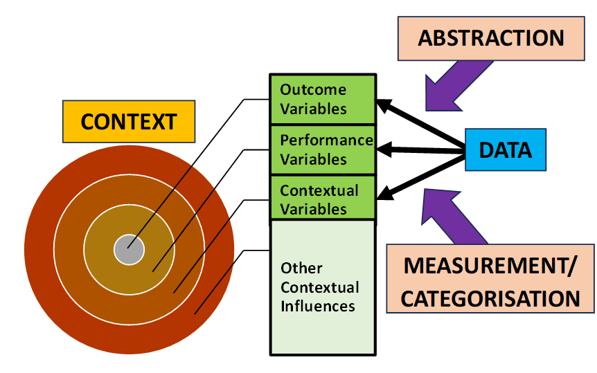
Analytical models takes the following general form:

Outcome = f(Performance, Context) + Stochastic Error

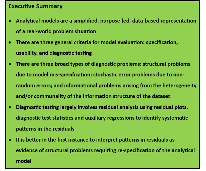
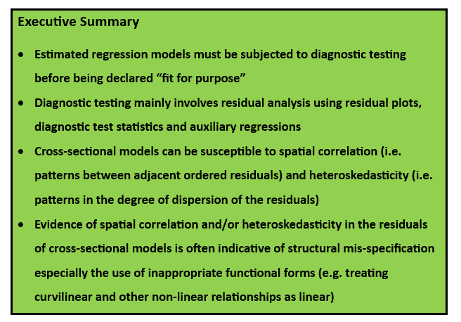
The structural model represents the systematic (or “global”) variation in the process outcome associated with the variation in the performance and context variables. The stochastic error acts as a sort of “garbage can” to capture “local” context-specific influences on process outcomes that are not generalisable in any systematic way across all the observations in the dataset. All analytical models assume that the structural model is well specified and the stochastic error is random. Diagnostic testing is the process of checking that these two assumptions hold true for any estimated analytical model.

Diagnostic testing involves the analysis of the residuals of the estimated analytical model.

Residual = Actual Outcome – Predicted Outcome

Diagnostic testing is the search for patterns in the residuals. It is a matter of interpretation as to whether any patterns in the residuals are due to structural mis-specification problems or stochastic error mis-specification problems. But structural problems must take precedence since, unless the structural model is correctly specified, the residuals will be biased estimates of the stochastic error since they will be contaminated by structural mis-specification. In this post I am focusing on structural mis-specification problems associated with cross-sectional data in which the dataset comprises observations of similar entities at the same point in time. I label this type of residual analysis as “spatial diagnostics”. I will utilise all three principal  methods for detecting systematic variation in residuals: residual plots, diagnostic test statistics, and auxiliary regressions.

Data

The dataset being used to illustrate spatial diagnostics was originally extracted from the Family Expenditure Survey in January 1993. The dataset contains information on 608 households. Four variables are used – weekly household expenditure (EXPEND) is the outcome variable to be modelled by weekly household income INCOME), the number of adults in the household (ADULTS) and the age of the head of the household (AGE) which is defined as whoever is responsible for completing the survey. The model is estimated using linear regression.

Initial Model

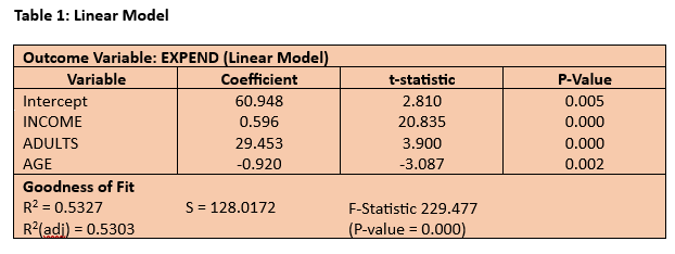
The estimated linear model is reported in Table 1 below. On the face of it, the estimated model seems satisfactory, particularly for such a simple cross-sectional model, with around 53% of the variation in weekly expenditure being explained statistically by variation in weekly income, the number of adults in the household and the age of the head of household (R2 = 0.5327). All three impact coefficients are highly significant (P-value < 0.01). The t-statistic provides a useful indicator of the relative importance of the three predictor variables since it effectively standardises the impact coefficients using their standard errors as a proxy for the units of measurement. Not surprisingly, weekly household expenditure is principally driven by weekly household income with, on average, 59.6p spent out of every additional £1 of income.

Diagnostic Tests

However, despite the satisfactory goodness of fit and high statistical significance of the impact coefficients, the linear model is not fit for purpose in respect of its spatial diagnostics. Its residuals are far from random as can be seen clearly in the two residual plots in Figures 1 and 2. Figure 1 is the scatterplot of the residuals against the outcome variable, weekly expenditure. The ideal would be a completely random scatterplot with no pattern in either the average value of the residual which should be zero (i.e. no spatial correlation) or in the degree of dispersion (known as “homoskedasticity”). In other words, the scatterplot should be centred throughout on the horizontal axis and there should also be a relatively constant vertical spread of the residual around the horizontal axis. But the residuals for the linear model are clearly trended upwards in both value (i.e. spatial correlation) and dispersion (i.e. heteroskedasticity). In most cases in my experience this sort of pattern in the residuals is caused by wrongly treating the core relationship as linear when it is better modelled as a curvilinear or some other form of non-linear relationship.

            Figure 2 provides an alternative residual plot in which the residuals are ordered by their associated weekly expenditure. Effectively this plot replaces the absolute values of weekly expenditure with their rankings from lowest to highest. Again we should ideally get a random plot with no discernible pattern between adjacent residuals (i.e. no spatial correlation) and no discernible pattern in the degree of dispersion (i.e. homoskedasticity). Given the number of observations and the size of the graphic it is impossible to determine visually if there is any pattern between the adjacent residuals in most of the dataset except in the upper tail. But the degree of spatial correlation can be measured by applying the correlation coefficient to the relationship between ordered residuals and their immediate neighbour. Any correlation coefficient > |0.5| represents a large effect. In the case of the ordered residuals for the linear model of weekly household expenditure the spatial correlation coefficient is 0.605 which provides evidence of a strong relationship between adjacent ordered residuals i.e. the residuals are far from random.

            So what is causing the pattern in the residuals? One way to try to answer this question is to estimate what is called an “auxiliary regression” in which regression analysis is applied to model the residuals from the original estimated regression model. One widely used form of auxiliary regression is to use the squared residuals as the outcome variable to be modelled. The results for this type of auxiliary regression applied to the residuals from the linear model of weekly household regression are reported in Table 2. The auxiliary regression overall is statistically significant (F = 7.755, P-value = 0.000). The key result is that there is a highly significant relationship between the squared residuals and weekly household income, suggesting that the next step is to focus on reformulating the income effect on household expenditure.

Revised Model and Diagnostic Tests

So diagnostic testing has suggested the strong possibility that modelling the income effect on household expenditure as a linear effect is inappropriate. What is to be done? Do we need to abandon linear regression as the modelling technique? Fortunately the answer is “not necessarily”. Although there are a number of non-linear modelling techniques, it is in most cases possible to continue using linear regression by transforming the original variables. Instead of changing the estimation method, the alternative is to transform the original variables such that there is a linear relationship between the transformed variables that is amenable to estimation by linear regression. One commonly used transformation is to introduce the square of a predictor alongside the original predictor to capture a quadratic relationship. Another common transformation is to convert the model into a loglinear form by using logarithmic transformations of the original variables. It is the latter approach that I have used as a first step in attempting to improve the structural specification of the household expenditure model. Specifically, I have replaced the original expenditure and income variables, EXPEND and INCOME, with their natural log transformations, LnEXPEND and LnINCOME, respectively. The results of the regression analysis and diagnostic testing of the new loglinear model are reported below.

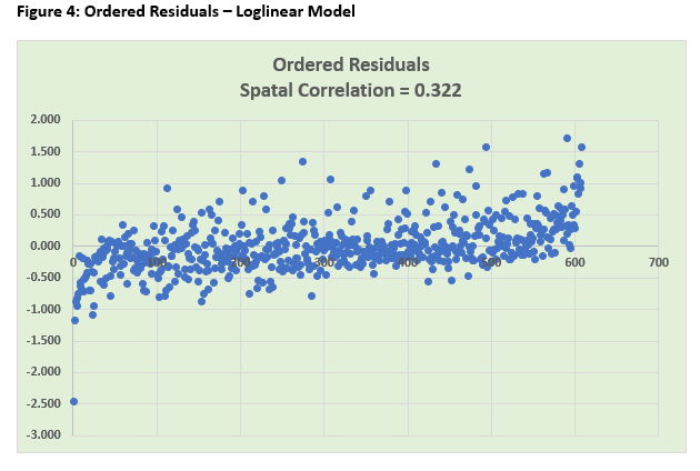
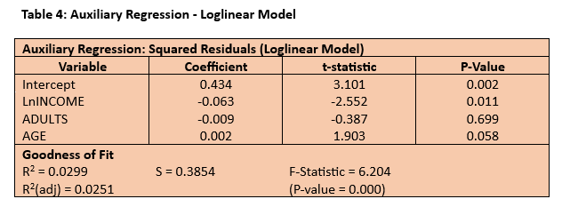
The estimated regression model is broadly similar in respect of its goodness of fit and statistical significance of the impact coefficients although, given the change in the functional form, these are not directly comparable. The impact coefficient on LnINCOME is 0.674 which represents what economists term “income elasticity” and implies that, on average, a 1% change in income is associated with a 0.67% change in expenditure in the same direction. The spatial diagnostics have improved although the residual scatterplot still shows evidence of a trend. The ordered residuals appear much more random than previously with the spatial correlation coefficient having been nearly halved and now evidence only of a medium-sized effect (> |0.3|) between adjacent residuals. The auxiliary regression is still significant overall (F = 6.204; P-value = 0.000) and, although the loglinear specification has produced a better fit for the income effect (with a lower t-statistic and increased P-value), it has had an adverse impact on the age effect (with a higher t-statistic and a P-value close to being significant at the 5% level). The conclusion – the regression model of weekly household expenditure remains “work in progress”. The next steps might be to consider extending the log transformation to the other predictors and/or introducing a quadratic age effect.

Other Related Posts

Diagnostic Testing Part 1: Why Is It So Important?

Diagnostic Testing Part 1: Why Is It So Important?

Analytical models are a simplified, purpose-led, data-based representation of a real-world problem situation. In terms of the categorisation of data proposed in the previous post, “Putting Data in Context” (24th Jan 2024), analytical models typical take the form of a multivariate relationship between the process outcome variable and a set of performance and context (i.e. predictor) variables.

Outcome = f(Performance, Context)

In evaluating the estimated models derived from a particular dataset, there are three general criteria to be considered:

  • Specification criterion: is the model as simple as possible but still comprehensive in its inclusion of all relevant variables?
  • Usability criterion: is the model fit for purpose?
  • Diagnostic testing criterion: does the model use the available data effectively?

These criteria are applicable to all estimated analytical models but the specific focus and empirical examples in this series of posts will be linear regression models.

Specification Criterion

Analytical models should only include as predictors the relevant performance and context variables that influence the (target) outcome variable. To keep the model as simple as possible, irrelevant variables with no predictive power should be excluded. In the case of linear regression models the adjusted R2 (i.e. adjusted for the number of variables and observations) is the most useful statistic for comparing the goodness of fit across linear regression models with different numbers of predictors. Maximising the adjusted R2 is equivalent to minimising the standard error of the regression and yields the model specification rule of retaining all predictors with (absolute) t-statistics > 1.

Usability Criterion

The purpose of an analytical model is to provide an evidential basis for developing an intervention strategy to improve process outcomes. There are three general requirements for a usable analytical model:

  • All systematic influences on process outcomes are included
  • Model goodness of fit is maximised
  • One or more predictor variables are controllable, that is, (i) causally linked to the process outcome; (ii) a potential target for managerial intervention; and (iii) with a sufficiently large effect size

Diagnostic Testing Criterion

A linear regression model takes the following general form:

Outcome = f(Performance, Context) + Stochastic Error

There are two components: (i) the structural model, f(.), that seeks to capture the systematic variation in the process outcome associated with the variation in the performance and context variables; and (ii) the stochastic error that represents the non-systematic variation in the process outcome. The stochastic error captures the myriad of “local” context-specific influences that impact on the individual observations but whose effects are not generalisable in any systematic way across all the observations in the dataset.

            Regression analysis, like all analytical models, assumes that (i) the structural model is well specified; and (ii) the stochastic error is random (which, in formal statistical terms, requires that the errors are identically and independently distributed). Diagnostic testing is the process of checking that these two assumptions hold true for any estimated analytical model. To use the signal-noise analogy from physics, data analytics can be seen as a signal-extraction process in which the objective is to separate the systematic information (i.e. signal) from the non-systematic information (i.e. noise). Diagnostic testing involves ensuring that all of the signal has been extracted and that the remaining information is random noise.

A Checklist of Possible Diagnostic Problems

There are three broad types of diagnostic problems:

  • Structural problems: these are potential mis-specification problems with the structural component of the analytical model and include wrong functional form, missing relevant variables, incorrect dynamics in time-series models, and structural instability (i.e. the estimated parameters are unstable across subsets of the data)
  • Stochastic error problems: the stochastic error is not well behaved and is non-independently and/or non-identically distributed
  • Informational problems: the information structure of the dataset is characterised by heterogeneity (i.e. outliers and/or clusters) and/or communality

Informational problems should be identified and resolved during the exploratory data analysis before estimating the analytical model. Diagnostic testing focuses on structural and stochastic error problems as part of the evaluation of estimated models. Within the diagnostic testing process, it is strongly recommended that priority is given to structural problems. Ultimately, as discussed below, diagnostic testing involves the analysis of the residuals of the estimated analytical model. Diagnostic testing is the search for patterns in the residuals. It is a matter of interpretation as to whether any patterns in the residuals are due to structural problems or stochastic error problems. But the solutions are quite different. Structural problems require that the structural component of the analytical model is revised whereas stochastic error problems require a different estimation method to be used. However, the residuals can only be “unbiased” estimates of the stochastic error if and only if the structural component is well specified. It comes down to mindset. If you have a “Master of the Universe” mindset and believe that the analytical model is well specified, then, from that perspective, any patterns in the residuals are a stochastic error problem requiring the use of more sophisticated estimation techniques. This is the traditional approach in econometrics by those wedded to the belief in the infallibility of mainstream economic theory and confident that theory-based models are well specified. In contrast, practitioners, if they are to be effective in achieving better outcomes, require a much greater degree of humility in the face of an uncertain world, recognising that analytical models are always fallible. Interpreting patterns in residuals as evidence of structural mis-specification is, in my experience, much more likely to lead to better, fit-for-purpose models.  

Diagnostic Testing as Residual Analysis  

Diagnostic testing largely involves the analysis of the residuals of the estimated analytical model.

Residual = Actual Outcome – Predicted Outcome

Essentially diagnostic testing is the search for patterns in the residuals. The most common types of patterns in residuals when ordered by size or time are correlations between successive residuals (i.e. spatial or serial correlation) and changes in their degree of dispersion  (known as “heteroskedasticity”). There are three principal methods for detecting systematic variation in residuals:

  • Residual plots – visualisations of the bivariate relationships between the residuals and the outcome and predictor variables
  • Diagnostic test statistics – formal hypothesis testing of the existence of systematic variation in the residuals
  • Auxiliary regressions – the estimation of supplementary regression models in which  as the outcome variable is the original (or transformed) residuals from the initial regression model

In subsequent posts I will review the use of residual analysis in both cross-sectional models (Part 2) and time-series models (Part 3). I will also consider the overfitting problem (Part 4) and structural instability (Part 5).

Other Related Posts

Putting Data in Context

Putting Data in Context

Executive Summary

  • Data analytics is data analysis for practical purpose so the context is necessarily the uncertain, unfolding future
  • Datasets consist of observations abstracted from relevant contexts and largely de-contextualised with only limited contextual information
  • Decisions must ultimately involve re-contextualising the results of data analysis using the knowledge and experience of the decision makers who have an intuitive, holistic appreciation of the specific decision context
  • Evidence of association between variables does not necessarily imply a causal relationship; causality is our interpretation and explanation of the association
  • Communality (i.e. shared information across variables) is inevitable in all datasets, reflecting the influence of context
  • There is always a “missing-variable” problem because datasets are always partial abstractions that simplify the real-world context of the data

As I argued in a previous post, “Analytics and Context” (9th Nov 2023), a deep appreciation of context is fundamental to data analytics. Indeed it is the importance of context that lay behind my use of the quote from the 19th Century Danish philosopher, Søren Kierkegaard, in the announcement of the latest set of posts on Winning With Analytics:

‘Life can only be understood backwards; but it must be lived forwards.’

Data analysis for the purpose of academic disciplinary research is motivated by the search for universality. Business disciplines such as economics, finance and organisational behaviour propose hypotheses about business behaviour and then test these hypotheses empirically. But the process of disciplinary hypothesis testing requires datasets in which the observations have been abstracted from individually unique contexts. Universality necessarily implies de-contextualising the data. Academic research is not about understanding the particular but rather it is about understanding the general. And the context is the past. We can only ever gather data about what has happened. As Kierkegaard so rightly said, ‘Life can only be understood backwards’.

Data analytics is data analysis for practical purpose so the context is necessarily the unfolding future. ‘Life must be lived forward.’ The dilemma for data analytics is that of life in general – uncertainty. There is no data for the future, just forecasts that ultimately assume in one way or another than the future will be like the past. Forecasts are extrapolations of varying degrees of sophistication, but extrapolations, nonetheless. So in providing actionable insights to guide the actions of decision makers, data analytics must always confront the uncertainty inherent in a world in constant flux. What this means in practical terms is that actionable insights derived from data analysis must be grounded in the particulars of the specific decision context. While data analysis whether for disciplinary or practical purposes always uses datasets consisting of observations abstracted from relevant contexts and largely de-contextualised, data analytics requires that the results of the data analysis are re-contextualised to take into account all of the relevant aspects of the specific decision context. Decisions must ultimately involve combining the results of data analysis with the knowledge and experience of the managers who have an intuitive, holistic appreciation of the specific decision context.

 Effective data analytics requires an understanding of the relationship between context and data which I have summarised below in Figure 1. The purpose of data analytics is to assist managers to understand the variation in the performance of those processes for which they have responsibility. Typically the analytics project is initiated by a managerial perception of underperformance and the need to decide on some form of intervention to improve future performance. The dataset to be analysed consists of three types of variables:

  • Outcome variables that categorise/measure the outcomes of the process under investigation;
  • Performance variables that categorise/measure aspects of the activities that constitute the process under investigation; and
  • Contextual variables that categorise/measure aspects of the wider context in which the process is operating

The dataset is an abstraction from reality (what I call a “realisation”) that provides only a partial representation of the outcome, performance and context of the process under investigation. This is what I meant by data always being de-contextualised to some extent. There will be a vast array of aspects of the process and its context that are excluded from the dataset but may in reality has some impact on the observed process outcomes (what I have labelled “Other Contextual Influences”).

            Not only is the dataset dependent on the specific criteria used to determine the information to be abstracted from the real-world context, but it is also dependent on the specific categorisation and measurement systems applied to that information. Categorisation is the qualitative representation of differences in type between the individual observations of a multi-type variable. Measurement is the quantitative representation of the degree of variation between the individual observations of a single-type variable.

Figure 1: The Relationship Between Context and Data

            When we use statistical tools to investigate datasets for evidence of relationships between variables, we must always remember that statistics can only ever provide evidence of association between variables in the sense of a consistent pattern in their joint variation. So, for example, when two measured variables are found to be positively associated, this means that there is a systematic tendency that as one of the variables changes, the other variable tends to change in the same direction. Association does not imply causality. At most association can provide evidence that is consistent with a causal relationship but never conclusive proof. Causality is our interpretation and explanation of the association. As we are taught in every introductory statistics class, statistical association between two variables, X and Y, can be consistent with one-way causality in either direction (X causing Y or Y causing X), two-way causality (X causing Y with a feedback loop from Y to X), “third-variable” causality i.e. the common causal effects of another variable, Z (Z causing both X and Y), or a spurious, non-causal relationship.

            When we recognise that datasets are abstractions from the real world that have been largely been decontextualised, there are two critical implications for the statistical analysis of the data. First, as I have argued in my previous post, “Analytics and Context”, there is no such thing as an independent variable. All variables in a dataset necessarily display what is called “communality”, that is, shared information reflecting the influence of their common context. There will always be some degree of contextual association between variables which makes it difficult to isolate the shape and size of the direct relationship between two variables. Statisticians refer to an association between supposedly independent variables as the “multicollinearity” problem. It is not really a problem, but rather a characteristic of every dataset. Communality implies that all bivariate statistical tests are always subject to bias due to the exclusion of the influence of other variables and the wider context. In practical terms, communality requires that exploratory data analysis should always include an exploration of the degree of association between the performance and contextual variables to be used to model the variation in the outcome variables. Communality also raises the possibility of restructuring the information in any dataset to consolidate shared information in new constructed variables using factor analysis. (This will be the subject of a future post.)

The second critical implication for statistical analysis is that there is always a “missing-variable” problem because datasets are always partial abstractions that simplify the real-world context of the data. Again, just like the so-called multicollinearity problem, the missing-variable problem is not really a problem but rather an ever-present characteristic of any dataset. It is the third-variable problem writ large. Other contextual influences have an indeterminate impact on the outcome variables and are always missing variables from he dataset. Of course, the usual response is that they are merely random, non-systematic influences captured by the stochastic error term included in any statistical model. But these stochastic errors are assumed to be independent which effectively just assumes away the problem. Contextual influences by their very nature are not independent from the variables in the dataset.

To conclude, communality and uncertainty (i.e. context) are ever-present characteristics of life that we need to recognise and appreciate when evaluating the results of data analysis in order to generate context-specific actionable insights that are fit for purpose.

Other Related Posts

Analytics and Context

Analytics and Context

Executive Summary

  • Context is crucial in data analytics because the purpose of data analytics is always practical to improve future performance
  • The context of a decision is the totality of the conditions that constitute the circumstances of the specific decision
  • The three key characteristics of the context of human behaviour in a social setting are (i) uniqueness; (ii) “infinitiveness”; and (iii) uncertainty
  • There are five inter-related implications for data analysts if they accept the critical importance of context:

Implication 1: The need to recognise that datasets and analytical models are always human-created “realisations” of the real world.

Implication 2: All datasets and analytical models are de-contextualised abstractions.

Implication 3: Data analytics should seek to generalise from a sample rather than testing the validity of universal hypotheses.

Implication 4: Given that every observation in a dataset is unique in its context, it is vital that exploratory data analysis investigates whether or not a dataset fulfils the similarity and variability requirements for valid analytical investigation.

Implication 5: It is misleading to consider analytical models as comprising dependent and independent variable

As discussed in a previous post, “What is data analytics?” (11th Sept 2023), data analytics is best defined as data analysis for practical purpose. The role of data analytics is to use data analysis to provide an evidential basis for managers to make evidence-based decisions on the most effective intervention to improve performance. Academics do not typically do data analytics since they are mostly using empirical analysis to pursue disciplinary, not practical, purposes. As soon as you move from disciplinary purpose to practical purpose, then context becomes crucial. In this post I want to explore the implications for data analytics of the importance of context.

              The principal role of management is to maintain and improve the performance levels of the people and resources for which they are responsible. Managers are constantly making decisions on how to intervene and take action to improve performance. To be effective, these decisions must be appropriate given the specific circumstances that prevail. This is what I call the “context” of the decision – the totality of the conditions that constitute the circumstances of the specific decision.

              In the case of human behaviour in a social setting, there are three key characteristics of the context:

  1.   Unique

Every context is unique. As Heraclitus famously remarked, “You can never step into the same river twice”. You as an individual will have changed by the time that you next step into the river, and the river itself will also have changed – you will not be stepping into the same water in the exactly the same place. So too with any decision context; however similar to previous decision contexts, there will some unique features including of course that the decision-maker will have experience of the decision from the previous occasion. In life, change is the only constant. From this perspective, there can never be universality in the sense of prescriptions on what to do for any particular type of decision irrespective of the specifics of the particular context. A decision is always context-specific and the context is always unique. 

2. “Infinitive”

By “infinitive” I mean that there are an infinite number of possible aspects of any given decision situation. There is no definitive set of descriptors that can capture fully the totality of the context of a specific decision.

3. Uncertainty

All human behaviour occurs in the context of uncertainty. We can never fully understand the past which will always remain contestable to some extent with the possibility of alternative explanations and interpretations. And we can never know in advance the full consequences of our decisions and actions because the future is unknowable. Treating the past and future as certain or probabilistic disguises but does not remove uncertainty. Human knowledge is always partial and fallible

              Much of the failings of data analytics derive from ignoring the uniqueness, “infinitiveness” and uncertainty of decision situations. I often describe it as the “Masters of the Universe” syndrome – the belief that because you know the numbers, you know with certainty, almost bordering on arrogance, what needs be done and all will be well with world if only managers would do what the analysts tell them to do. This lack of humility on the part of analysts puts managers offside and typically leads to analytics being ignored. Managers are experts in context. Their experience has given them an understanding, often intuitive, of the impact of context. Analysts should respect this knowledge and tap into it. Ultimately the problem lies in treating social human beings who learn from experience as if they behave in a very deterministic manner similar to molecules. The methods that have been so successful in generating knowledge in the natural sciences are not easily transferable to the realm of human behaviour. Economics has sought to emulate the natural sciences in adopting a scientific approach to the empirical testing of economic theory. This has had an enormous impact, sometimes detrimental, on the mindset of data analysts given that a significant number of data analysts have a background in economics and econometrics (i.e. the application of statistical analysis to study of economic data).

              So what are the implications if we as data analysts accept the critical importance of context? I would argue there are five inter-related implications:

Implication 1: The need to recognise that datasets and analytical models are always human-created “realisations” of the real world.

The “infinitiveness” of the decision context implies that datasets and analytical models are always partial and selective. There are no objective facts as such. Indeed the Latin root of the word “fact” is facere (“to make”). Facts are made. We frame the world, categorise it and measure it. Artists have always recognised that their art is a human interpretation of the world. The French impressionist painter, Paul Cezanne, described his paintings as “realisations” of the world. Scientists have tended to designate their models of the world as objective which tends to obscure their interpretive nature. Scientists interpret the world just as artists do, albeit with very different tools and techniques. Datasets and analytical models are the realisations of the world by data analysts.

Implication 2: All datasets and analytical models are de-contextualised abstractions.

As realisations, datasets and analytical models are necessarily selective, capturing only part of the decision situation. As such they are always abstractions from reality. The observations recorded in a dataset are de-contextualised in the sense that they are abstracted from the totality of the decision context.

Implication 3: Data analytics should seek to generalise from a sample rather that testing the validity of universal hypotheses.

There are no universal truths valid across all contexts. The disciplinary mindset of economics is quite the opposite. Economic behaviour is modelled as constrained optimisation by rational economic agents. Theoretical results are derived formally by mathematical analysis and their validity in specific contexts investigated empirically, in much the same way as natural science uses theory to hypothesise outcomes in laboratory experiments. Recognising the unique, “infinitive” and uncertain nature of the decision context leads to a very different mindset, one based on intellectual humility and the fallibility of human knowledge. We try to generalise from similar previous contexts to unknown, yet to occur, future contexts. These generalisations are, by their very nature, uncertain and fallible.

Implication 4: Given that every observation in a dataset is unique in its context, it is vital that exploratory data analysis investigates whether or not a dataset fulfils the similarity and variability requirements for valid analytical investigation.

Every observation in a dataset is an abstraction from a unique decision context. One of the critical roles of the Exploration stage of the analytics process is to ensure that the decision contexts of each observation are sufficiently similar to be treated as a single collective (i.e. sample) to be analysed. The other side of the coin is checking the variability. There needs to be enough variability between the decision contexts so that the analyst can investigate which aspects of variability in the decision contexts are associated with the variability in the observed outcomes. But if the variability is excessive, this may call into question the degree of similarity and whether or not it is valid to assume that all of the observations have been generated by the same general behaviour process. Excessive variability (e.g. outliers) may represent different behavioural processes, requiring the dataset to be analysed as a set of sub-samples rather than as a single sample.

Implication 5: It can be misleading to consider analytical models as comprising dependent and independent variables.

Analytical models are typically described in statistics and econometrics as consisting of dependent and independent variables. This embodies a rather mechanistic view of the world in which the variation of observed outcomes (i.e. the dependent variable) is to be explained by the variation in the different aspects of the behavioural process as measured (or categorised) by the independent variables. But in reality these independent variables are never completely independent of each other. They share information (often known as “commonality”) to the extent that for each observation the so-called independent variables are extracted from the same context. I prefer to think of the variables in a dataset as situational variables – they attempt to capture the most relevant aspects of the unique real-world situations from which the data has been extracted but with no assumption that they are independent; indeed quite the opposite. And, given the specific practical purpose of the particular analytics project, one or more of these situational variables will be designated as outcome variables.

Read Other Related Posts

What is Data Analytics? 11th Sept 2023

The Six Stages of the Analytics Process, 20th Sept 2023

Measuring Trend Growth

Executive Summary

  • The most useful summary statistic for a trended variable is the average growth rate
  • But there are several different methods for calculating average growth rates that can often generate very different results depending on whether all the data is used or just the start and end points, and whether simple or compound growth is assumed
  • Be careful of calculating average growth rates using only the start and end points of trended variables since this implicitly assumes that these two points are representative of the dynamic path of the trended variable and may give a very biased estimate of the underlying growth rate
  • Best practice is to use all of the available data to estimate a loglinear trendline which allows for compound growth and avoids having to calculate an appropriate midpoint of a linear trendline to convert the estimated slope into  growth rate

When providing summary statistics for trended time-series data, the mean makes no sense as a measure of the point of central tendency. By definition, there is no point of central tendency in trended data. Trended data are either increasing or decreasing in which case the most useful summary statistic is the average rate of growth/decline. But how do you calculate the average growth rate? In this post I want to discuss the pros and cons of the different ways of calculating the average growth rate, using total league attendances in English football (the subject of my previous post) as an illustration.

              There are at least five different methods of calculating the average growth rate:

  1. “Averaged” growth rate: use gt = (yt – yt-1)/yt-1 to calculate the growth rate for each period then average these growth rates
  2. Simple growth rate: use the start and end values of the trended variable to calculate the simple growth rate with the trended variable modelled as yt+n = yt(1 + ng)
  3. Compound growth rate: use the start and end values of the trended variable to calculate the compound growth rate with the trended variable modelled as yt+n = yt(1 + g)n
  4. Linear trendline: estimate the line of best fit for yt = a + gt (i.e. simple growth)
  5. Loglinear trendline: estimate the line of best fit for ln yt = a + gt (i.e. compound growth)

where y = the trended variable; g  = growth rate; t = time period; n = number of time periods; a = intercept in line of best fit

These methods differ in two ways. First, they differ as to whether the trend is modelled as simple growth (Methods 2, 4) or compound growth (Methods 3, 5). Method 1 is effectively neutral in this respect. Second, the methods differ in terms of whether they use only the start and end points of the trended variable (Methods 2, 3) or use all of the available data (Methods 1, 4, 5). The problem with only using the start and end points is that there is an implicit assumption that these are representative of the underlying trend with relatively little “noise”. But this is not always the case and there is a real possibility of these methods biasing the average growth rate upwards or downwards as illustrated by the following analysis of the trends in football league attendances in England since the end of the Second World War.

Figure 1: Total League Attendances (Regular Season), England, 1946/47-2022/23

This U-shaped timeplot of total league attendances in England since the end of the Second World War splits into two distinct sub-periods of decline/growth:

  • Postwar decline: 1948/49 – 1985/86
  • Current revival: 1985/86 – 2022/23

Applying the five methods to calculate the average annual growth rate of these two sub-periods yields the following results:

MethodPostwar Decline 1948/49 – 1985/86Current Revival 1985/86 – 2022/23*
Method 1: “averaged” growth rate-2.36%2.28%
Method 2: simple growth rate-1.62%3.00%
Method 3: compound growth-2.45%2.04%
Method 4: linear trendline-1.89%1.75%
Method 5: loglinear trendline-1.95%1.85%
*The Covid-affected seasons 2019/20 and 2020/21 have been excluded from the calculations of the average growth rate.

What the results show very clearly is the wide variability in the estimates of average annual growth rates depending on the method of calculation. The average annual rate of decline in league attendances between 1949 and 1986 varies between -1.62% (Method 2 – simple growth rate) to -2.45% (Method 3 – compound growth rate). Similarly the average annual rate of growth from 1986 onwards ranges from 1.75% (Method 4 – linear trendline) to 3.00% (Method 2 – simple growth rate). To investigate exactly why the two alternative methods for calculating the simple growth rate during the Current Revival give such different results, the linear trendline for 1985/86 – 2022/23 is shown graphically in Figure 2.

Figure 2: Linear Trendline, Total League Attendances, England, 1985/86 – 2022/23

As can be seen, the linear trendline has a high goodness of fit (R2 = 93.1%) and the fitted endpoint is very close to the actual gate attendance of 34.8 million in 2022/23. However, there is a relatively large divergence at the start of the period with the fitted trendline having a value of 18.2 million whereas the actual gate attendance in 1985/86 was 16.5 million. It is this divergence that accounts in part for the very different estimates of average annual growth rate generated by the two methods despite both assuming a simple growth rate model. (The rest of the divergence is due to the use of midpoint to convert the slope of the trendline into a growth rate.)

              So which method should be used? My advice is to be very wary of calculating average growth rates using only the start and end points of trended variables. You are implicitly assuming that these two points are representative of the dynamic path of the trended variable and may give a very biased estimate of the underlying growth rate. My preference is always to use all of the available data to estimate a loglinear trendline which allows for compound growth and avoids having to calculate an appropriate midpoint of a linear trendline to convert the estimated slope into a growth rate.

Read Other Related Posts

The Problem with Outliers

Executive Summary

  • Outliers are unusually extreme observations that can potentially cause two problems:
    1. Invalidating the homogeneity assumption that all of the observations have been generated by the same behavioural processes; and
    2. Unduly influencing any estimated model of the performance outcomes
  • A crucial role of exploratory data analysis is to identify possible outliers (i.e. anomaly detection) to inform the modelling process
  • Three useful techniques for identifying outliers are exploratory data visualisation, descriptive statistics and Marsh & Elliott outlier thresholds
  • It is good practice to report estimated models including and excluding the outliers in order to understand their impact on the results

A key function of the Exploratory stage of the analytics process is to understand the distributional properties of the dataset to be analysed. Part of the exploratory data analysis is to ensure that the dataset meets both the similarity and variability requirements. There must be sufficient similarity in the data to make it valid to treat the dataset as homogeneous with all of the observed outcomes being generated by the same behavioural processes (i.e. structural stability). But there must also be enough variability in the dataset both in the performance outcomes and the situational variables potentially associated with the outcomes so that relationships between changes in the situational variables and changes in performance outcomes can be modelled and investigated.

Outliers are unusually extreme observations that call into question the homogeneity assumption as well as potentially having an undue influence on any estimated model. It may be that the outliers are just extreme values generated by the same underlying behavioural processes as the rest of the dataset. In this case the homogeneity assumption is valid and the outliers will not bias the estimated models of the performance outcomes. However, the outliers may be the result of very different behavioural processes, invalidating the homogeneity assumption and rendering the estimated results of limited value for actionable insights. The problem with outliers is that we just do not know whether or not the homogeneity assumption is invalidated. So it is crucial that the exploratory data analysis identifies possible outliers (what is often referred to as “anomaly detection”) to inform the modelling strategy.

The problem with outliers is illustrated graphically below. Case 1 is the baseline with no outliers. Note that the impact (i.e. slope) coefficient of the line of best fit is 1.657 and the goodness of fit is 62.9%.

Case 2 is what I have called “homogeneous outliers” in which a group of 8 observations have been included that have unusually high values but have been generated by the same behavioural process as the baseline observations. In other words, there is structural stability across the whole dataset and hence it is legitimate to estimate a single line of best fit. Note that the inclusion of the outliers slightly increases the estimated impact coefficient to 1.966  but the goodness of fit increases substantially to 99.6%, reflecting the massive increase in the variance of the observations “explained” by the regression line.

Case 3 is that of “heterogeneous outliers” in which the baseline dataset has now been expanded to include a group of 8 outliers generated by a very different behavioural process. The homogeneity assumption is no longer valid so it is inappropriate to model the dataset with a single line of best fit. If we do so, then we find that the outliers have an undue influence with the impact coefficient now estimated to be 5.279, more than double the size of the estimated impact coefficient for the baseline dataset excluding the outliers. Note that there is a slight decline in the goodness of fit to 97.8% in Case 3 compared to Case 2, partly due to the greater variability of the outliers as well as the slightly poorer fit for the baseline observations of the estimated regression line.

Of course, in this artificially generated example, it is known from the outset that the outliers have been generated by the same behavioural process as the baseline dataset in Case 2 but not in Case 3. The problem we face in real-world situations is that we do not know if we are dealing with Case 2-type outliers or Case 3-type outliers. We need to explore the dataset to determine which is more likely in any given situation.

There are a number of very simple techniques that can be used to identify possible outliers. Three of the most useful are:

  1. Exploratory data visualisation
  2. Summary statistics
  3. Marsh & Elliott outlier thresholds

1.Exploratory data visualisation

Histograms and scatterplots as always should be the first step in any exploratory data analysis to “eyeball” the data and get a sense of the distributional properties of the data and the pairwise relationships between all of the measured variables.

2.Summary statistics

Descriptive statistics provide a formalised summary of the distributional properties of variables. Outliers at one tail of the distribution will produce skewness that will result n a gap between the mean and median. If there are outliers in the upper tail, this will tend to inflate the mean relative to the median (and the reverse if the outliers are in the lower tail). It is also useful to compare the relative dispersion of the variables. I always include the coefficient of variation (CoV) in the reported descriptive statistics.

CoV = Standard Deviation/Mean

CoV uses the mean to standardise the standard deviation for differences in measurement scales so that the dispersion of variables can be compared on a common basis. Outliers in any particular variable will tend to increase CoV relative to other variables.

3. Marsh & Elliott outlier thresholds

Marsh & Elliott define outliers as any observation that lies more than 150% of the interquartile range beyond either the first quartile (Q1) or the third quartile (Q3).

Lower outlier threshold: Q­1 – [1.5(Q3 – Q1)]

Upper outlier threshold: Q­3 + [1.5(Q3 – Q1)]

I have found these thresholds to be useful rules of thumb to identify possible outliers.

Another very useful technique for identifying outliers is cluster analysis which will be the subject of a later post.

So what should you do if the exploratory data analysis indicates the possibility of outliers in your dataset? As the artificial example illustrated, outliers (just like multicollinearity) need not necessarily create a problem for modelling a dataset. The key point is that exploratory data analysis should alert you to the possibility of problems so that you are aware that you may need to take remedial actions when investigating the multivariate relationships between outcome and situational variables at the Modelling stage. It is good practice to report estimated models including and excluding the outliers in order to understand their impact on the results. If there appears to be a sizeable difference in one or more of the estimated coefficients when the outliers are included/excluded, then you should formally test for structural instability using F-tests (often called Chow tests). Testing for structural stability in both cross-sectional and longitudinal/time-series data will be discussed in more detail in a future post. Some argue to drop outliers from the dataset but personally I am loathe to discard any data which may contain useful information. Knowing the impact of the outliers on the estimated coefficients can be useful information and, indeed, it may be that further investigation into the specific conditions of the outliers could prove to be of real practical value.

The two main takeaway points are that (1) a key component of exploratory data analysis should always be checking for the possibility of outliers; and (2) if there are outliers in the dataset, ensure that you investigate their impact on the estimated models you report. You must avoid providing actionable insights that have been unduly influenced by outliers that are not representative of the actual situation with which you are dealing.

Read Other Related Posts

Competing on Analytics

Executive Summary

  • Tom Davenport, the management guru on data analytics, defines analytics competitors as organisations committed to quantitative, fact-based analysis
  • Davenport identifies five stages in becoming an analytical competitor: Stage 1: Analytically impaired Stage 2: Localised analytics Stage 3: Analytical aspirations Stage 4: Analytical companies Stage 5: Analytical competitors
  • In Competing on Analytics: The New Science of Winning, Davenport and Harris identify four pillars of analytical competition: distinctive capability; enterprise-wide analytics; senior management commitment; and large-scale ambition
  • The initial actionable insight that data analytics can help diagnose why an organisation is currently underperforming and prescribe how its future performance can be improved is the starting point of the analytical journey

Over the last 20 years, probably the leading guru on the management of data analytics in organisations has been Tom Davenport. He came to prominence with his article “Competing on Analytics” (Harvard Business Review, 2006) followed up in 2007 by the book, Competing on Analytics: The New Science of Winning (co-authored with Jeanne Harris). Davenport’s initial study focused on 32 organisations that had committed to quantitative, fact-based analysis, 11 of which he designated as “full-bore analytics competitors”. He identified three key attributes of analytics competitors:

  • Widespread use of modelling and optimisation
  • An enterprise approach
  • Senior executive advocates

Davenport found that analytics competitors had four sources of strength – the right focus, the right culture, the right people and the right technology. In the book, he distilled these characteristics of analytic competitors into the four pillars of analytical competition:

  • Distinctive capability
  • Enterprise-wide analytics
    • Senior management commitment
  • Large-scale ambition

Davenport identifies five stages in becoming an analytical competitor:

  • Stage 1: Analytically impaired
  • Stage 2: Localised analytics
  • Stage 3: Analytical aspirations
  • Stage 4: Analytical companies
  • Stage 5: Analytical competitors

Davenport’s five stages of analytical competition

Stage 1: Analytically Impaired

At Stage 1 organisations make negligible use of data analytics. They are not guided by any performance metrics and are essentially “flying blind”. What data they have are poor quality, poorly defined and unintegrated. Their analytical journey starts with the question of what is happening in their organisation that provides the driver to get more accurate data to improve their operations. At this stage, the organisational culture is “knowledge-allergic” with decisions driven more by gut-feeling and past experience rather than evidence.

Stage 2: Localised Analytics

Stage 2 sees analytics being pioneered in organisations by isolated individuals concerned with improving performance in those local aspects of the organisation’s operations with which they are most involved. There is no alignment of these initial analytics projects with overall organisational performance. The analysts start to produce actionable insights that are successful in improving performance. These local successes begin to attract attention elsewhere in the organisation. Data silos emerge with individuals creating datasets for specific activities and stored in spreadsheets. There is no senior leadership recognition at this stage of the potential organisation-wide gains from analytics.

Stage 3: Analytical Aspirations

Stage 3 in many ways marks the “big leap forward” with organisations beginning to recognise at a senior leadership level that there are big gains to be made from employing analytics across all of the organisation’s operations. But there is considerable resistance from managers with no analytics skills and experience who see their position as threatened. With some senior leadership support there is an effort to create more integrated data systems and analytics processes. Moves begin towards a centralised data warehouse managed by data engineers.

Stage 4: Analytical Companies

By Stage 4 organisations are establishing a fact-based culture with broad senior leadership support. The value of data analytics in these organisations is now generally accepted. Analytics processes are becoming embedded in everyday operations and seen as an essential part of “how we do things around here”. Specialist teams of data analysts are being recruited and managers are becoming familiar with how to utilise the results of analytics to support their decision making. There is a clear strategy on the collection and storage of high-quality data centrally with clear data governance principles in place.

Stage 5: Analytical Competitors

At Stage 5 organisations are now what Davenport calls “full-bore analytical competitors” using analytics not only to improve current performance of all of the organisation’s operations but also to identify new opportunities to create new sustainable competitive advantages. Analytics is seen as a primary driver of organisational performance and value. The organisational culture is fact-based and committed to using analytics to test and develop new ways of doing things.

To quote an old Chinese proverb, “a thousand-mile journey starts with a single step”. The analytics journey for any organisation starts with an awareness that the organisation is underperforming and data analytics has an important role in facilitating an improvement in organisational performance. The initial actionable insight that data analytics can help diagnose why an organisation is currently underperforming and prescribe how its performance can be improved in the future is the starting point of the analytical journey.

Read Other Related Posts

The Keys to Success in Data Analytics

Executive Summary

  • Data analytics is a very useful servant but a poor leader
  • There are seven keys to using data analytics effectively in any organisation:
  1. A culture of evidence-based practice
  2. Leadership buy-in
  3. Decision-driven analysis
  4. Recognition of analytics as a source of marginal gains
  5. Realisation that analytics is more than reporting outcomes
  6. Soft skills are crucial
  7. Integration of data silos
  • Effective analysts are not just good statisticians
  • Analysts must be able to engage with decision-makers and “speak their language”

Earlier this year, I gave a presentation to a group of data analysts in a large organisation. My remit was to discuss how data analytics can be used to enhance performance. They were particularly interested in the insights I had gained from my own experience both in business (my career started as an analyst in the Unilever’s Economics Department in the mid-80s) and in elite team sports. I started off with my basic philosophy that “data analytics is a very useful servant but a poor leader” and then summarised the lessons I had learnt as seven keys to success in data analytics. Here are those seven keys to success.

1.A culture of evidence-based practice

Data analytics can only be effective in organisations committed to evidence-based practice. Using evidence to inform management decisions to enhance performance must be part of the corporate culture, the organisation’s way of doing things. The culture must be a process culture by which I mean a deep commitment to doing things the right way. In a world of uncertainty we can never be sure that what we do will lead to the future outcomes we want and expect. We can never fully control future outcomes. Getting the process right in the sense of using data analytics to make the effective use of all the available evidence will maximise the likelihood of an organisation achieving better performance outcomes.

2. Leadership buy-in

A culture of evidence-based practice can only thrive when supported and encouraged by the organisation’s leadership. A “don’t do as I do, do as I say” approach seldom works. Leaders must lead by example and continually demonstrate and extol the virtues of evidence-based practice. If a leader adopts the attitude that “I don’t need to know the numbers to know what the right thing is to do” then this scepticism about the usefulness of data analytics will spread throughout the organisation and fatally undermine the analytics function.

3. Decision-driven analysis

Data analytics is data analysis for practical purpose. The purpose of management one way or another is to improve performance. Every data analytics project must start with the basic question “what managerial decision will be impacted by the data analysis?”. The answer to the question gives the analytics project its direction and ensures its relevance. The analyst’s function is not to find out things that they think would be interesting to know but rather things that the manager needs to know to improve performance.

4. Recognition of analytics as a source of marginal gains

The marginal gains philosophy, which emerged in elite cycling, is the idea that making a large improvement in performance is often achieved as the cumulative effect of lots of small changes. The overall performance of an organisation involves a myriad of decisions and actions. Data analytics can provide a structured approach to analysing organisational performance, decomposing it into its constituent micro components, benchmarking these micro performances against past performance levels and the performance levels of other similar entities, and identifying the performance drivers. Continually searching for marginal gains fosters a culture of wanting to do better and prevents organisational complacency.

5. Realisation that analytics is more that reporting outcomes

In some organisations data analytics is considered mainly as a monitoring process, tasked with tracking key performance indicators (KPIs) and reporting outcomes often visually with performance dashboards. This is an important function in any organisation but data analytics is much more than just monitoring performance. Data analytics should be diagnostic, investigating fluctuations in performance and providing actionable insights on possible managerial interventions to improve performance.

6. Soft skills are crucial

Effective analysts must have the “hard” skills of being good statisticians, able to apply appropriate analytical techniques correctly. But crucially effective analysts must also have the “soft” skills of being able to engage with managers and speak their language. Analysts must understand the managerial decisions that they are expected to inform, and they must be able to tap into the detailed knowledge of managers. Analysts must avoid being seen as the “Masters of the Universe”. They must respect the managers, work for them and work with them. Analysts should be humble. They must know what they bring to the table (i.e. the ability to forensically explore data) and what they don’t (i.e. experience and expertise of the specific decision context). Effective analytics is always a team effort.

7. Integration of data silos

Last but not least, once data analytics has progressed in an organisation beyond a few individuals working in isolation and storing the data they need in their own spreadsheets, there needs to be a centralised data warehouse managed by experts in data management. Integrating data silos opens up new possibilities for insights. This is a crucial part of an organisation developing the capabilities of an “analytical competitor” which I will explore in my next Methods post.

Read Other Related Posts

The Six Stages of the Analytics Process

Executive Summary

  • The analytics process can be broken down further into six distinct stages:  (1) Discovery; (2) Exploration; (3) Modelling; (4) Projection; (5) Actionable Insight; and (6) Monitoring
  • Always start the analytics process with the question: “What is the decision that will be impacted by the analysis?”
  • There are three principal pitfalls in deriving actionable insights from analytical models – generalisability, excluded-variable bias, and misinterpreting causation

The analytics process can be broken down further into six distinct stages:

  1. Discovery
  2. Exploration
  3. Modelling
  4. Projection
  5. Actionable Insight
  6. Monitoring
Figure 1: The Six Stages of the Analytics Process

Stage 1: Discovery

The discovery stage starts with a dialogue between the analyst and decision maker to ensure that the analyst understands the purpose of the project. Particular attention is paid to the specific decisions for which the project is intended to provide an evidential basis to support management decision making.

The starting point for all analytics projects is discovery. The Discovery stage involves a dialogue with the project sponsor to understand both Purpose (i.e. what is expected from the project?) and Context (i.e. what is already known?). The outcome of discovery is Framing the practical management problem facing the decision-maker as an analytical problem amenable to data analysis. It is crucial to ensure that the analytical problem is feasible given the available data.

Stage 2: Exploration

The exploration stage involves data preparation particularly checking the quality of the data and transforming the data if necessary. A key part of this exploration stage is the preliminary assessment of the basic properties of the data to decide on the appropriate analytical methods to be used in the modelling stage.

Having determined the purpose of the analytics project and sourced the relevant data in the initial Discovery stage, there is a need to gain a basic understanding of the properties of the data. This exploratory data analysis serves a number of ends:

  • It will help identify any problems in the quality of the data such as missing and suspect values.
  • It will provide an insight into the amount of information contained in the dataset (this will ultimately depend on the similarity and variability of the data).
  • If done effectively, exploratory data analysis will give clear guidance on how to proceed in the third Modelling stage.
  • It may provide advance warning of any potential statistical difficulties.

A dataset contains multiple observations of performance outcome and associated situational variables that attempt to capture information about the context of the performance. For the analysis of the dataset to produce actionable insights, there is both a similarity requirement and a variability requirement. The similarity requirement is that the dataset is structurally stable in the sense that it contains data on performance outcomes produced by a similar behaviour process across different entities (i.e. cross-sectional data) or across time (i.e. longitudinal data). The similarity requirement also requires that there is consistent measurement and categorisation of the outcome and situational variables. The variability requirement is that the dataset contains sufficient variability to allow analysis of changes in performance but without excessive variability that would raise doubts about the validity of treating the dataset as structurally stable.

Stage 3: Modelling

The modelling stage involves the construction of a simplified, purpose-led, data-based representation of the specific aspect of real-world behaviour on which the analytics project will focus.

The Modelling stage involves the use of statistical analysis to construct an analytical model of the specific aspect of real-world behaviour with which the analytics project is concerned. The analytical model is a simplified, purpose-led, data-based representation of the real-world problem situation.

  • Purpose-led: model design and choice of modelling techniques are driven by the analytical purpose (i.e. the management decision to be impacted by the analysis)
  • Simplified representation: models necessarily involve abstraction with only relevant, systematic features of the real-world decision situation included in the model
  • Data-based: modelling is the search for congruent models that best fit the available data and capture all of the systematic aspects of performance

The very nature of an analytical model creates a number of potential pitfalls which can lead to: (i) misinterpretation of the results of the data analysis; and (ii) misleading inferences as regards action recommendations. There are three principal pitfalls:

  • Generalisability: analytical models are based on a limited sample of data but actionable insights require that the results of the data analysis are generalisable to other similar contexts
  • Excluded-variable bias: analytical models are simplifications of reality that only focus on a limited number of variables but the reliability of the actionable insights demands that all relevant, systematic drivers of the performance outcomes are included otherwise the results may be statistically biased and misleading
  • Misinterpreting causation: analytical models are purpose-led so there is a necessity that the model captures causal relationships that allow for interventions to resolve practical problems and improve performance but statistical analysis can only identify associations; causation is ultimately a matter of interpretation

It is important to undertake diagnostic testing to try to avoid these pitfalls.

Stage 4: Projection

The projection stage involves using the estimated models developed in the modelling stage to answer what-if questions regarding the possible consequences of alternative interventions under different scenarios. It also involves forecasting future outcomes based on current trends.

Having constructed a simplified, purpose-led model of the business problem in the Modelling stage, the Projection stage involves using this model to answer what-if questions regarding the possible consequences of alternative interventions under different scenarios. The use of forecasting techniques to project future outcomes based on current trends is a key aspect of the Projection stage.

There are two broad types of forecasting methods:

  • Quantitative (or statistical) methods of forecasting e.g. univariate time-series models; causal models; Monte Carlo simulations
  • Qualitative methods e.g. Delphi method of asking a panel of experts; market research; opinion polls

Stage 5: Actionable insight

During this stage the analyst presents an evaluation of the alternative possible interventions and makes recommendations to the decision maker.

Presentations and business reports should be designed to be appropriate for the specific audience for which they are intended. A business report is typically structured into six main parts: Executive Summary; Introduction; Main Report; Conclusions; Recommendations; Appendices. Data visualisation can be a very effective communication tool in presentations and business reports and is likely to be much more engaging than a sets of bullet points but care should be taken to avoid distorting or obfuscating the patterns in the data. Effective presentations must have a clear purpose and be well planned and well-rehearsed.

Stage 6: Monitoring

The Monitoring stage involves tracking the project Key Performance Indicators (KPIs) during and after implementation.

The implementation plans for projects should, if possible, have decision points built into them. These decision points provide the option to alter the planned intervention if there is any indication that there have been structural changes in the situation subsequent to the original decision. Hence it is important to track the project KPIs during and after implementation to ensure that targeted improvements in performance are achieved and continue to be achieved. Remember data analytics does not end with recommendations for action. Actionable insights should always include recommendations on how the impact of the intervention on performance will be monitored going forward. Dashboards can be a very effective visualisation for monitoring performance.

Read other Related Posts

What is Data Analytics?

Executive Summary

  • Data analytics is data analysis for practical purpose
  • The three D’s of analytics are Decision, Domain and Data
  • Data analytics is a key component of an evidence-based approach to decision making
  • Data analytics consists of four modes – exploration (descriptive), modelling (diagnostic), projection (predictive) and decision (prescriptive)

Data analytics is a much used descriptor these days with its own myths and legends, usually of its successes.  The best known of these analytics myths and legends include exploding manholes, vintage wine, pregnant teenagers, Moneyball, Google Flu and Hollywood blockbusters. But what is data analytics?

A useful starting point is Wikipedia’s definition that data analytics is “the discovery and communication of meaningful patterns in data” which highlights the importance of communication. Data analytics is not just data analysis but also the effective presentation of these results. Data analytics always revolves around its intended audience. My own preferred definition is that data analytics is data analysis for practical purpose. This definition puts the stress on practical purpose. Being an empirically-minded academic in a business school, I am surrounded by data analysis but, much to the consternation of some of my colleagues, I have often said that academics don’t tend to do data analytics. Data analysis in business schools like other university faculties, especially in the social sciences, is primarily geared towards developing the academic discipline by publishing peer-reviewed journal articles. Data analytics is data analysis for practical, not disciplinary, purpose. Academic research does not necessarily produce actionable insights whereas the whole point of data analytics is to provide an evidential basis for decisions on what to do. Effective data analytics is always what I now call “impact theory” – using data to understand the world in order to intervene to change the world for the better. Analytics as impact theory is the guiding vision of Winning With Analytics.

Data analytics can be summed up the three D’s – Decision, Domain and Data. Data analytics is driven by the purpose of informing decisions by providing an evidential basis for decision makers to decide on the best available intervention to improve performance. Data analytics can only be effective if the data analysis is contextualised so that the practical recommendations are appropriate for the specific domain in which the decision makers are operating. And data analytics by definition involves the analysis of data but that analysis must be driven by the decision and domain, hence why data is listed last of the three D’s.

The essence of data analytics is improving performance by knowing your numbers. Whatever type of organisation – business, sport, public service or social – and irrespective of the level within the organisation, management is all about facilitating an improvement in performance. Management is about getting the best out people (i.e. efficacy) and the most out of the available resources (i.e. efficiency). Ultimately, data analytics is about producing actionable insight to improve efficacy and efficiency.

Data analytics is often seen as just reporting key performance indicators (KPIs). Reporting KPIs is one of the tasks of business intelligence. But data analytics is much more than reporting KPIs. Indeed one important task of data analytics is to identify the most useful set of KPIs. (The choice of KPIs will be the subject of a future post.) The various roles of data analytics can be summarised by the four modes of analytics:

  1. Exploration (what has been the level of performance?) – the descriptive role of summarising performance using descriptive statistics and data visualisation
  2. Modelling (why has performance changed?) – the diagnostic role of forensically investigating the causes of variation in performance levels
  3. Projection (how could performance be improved?) – the predictive role of projecting future performance based on recent performance trends and possible interventions
  4. Decision (what should be done?) – the prescriptive role of recommendations on the most appropriate intervention to improve current performance levels