January 2024 – Winning With Analytics

Diagnostic Testing Part 1: Why Is It So Important?

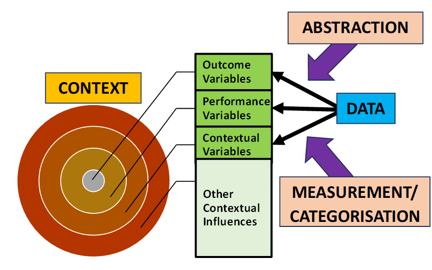
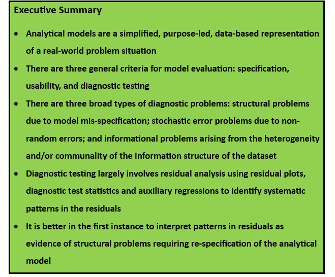
Analytical models are a simplified, purpose-led, data-based representation of a real-world problem situation. In terms of the categorisation of data proposed in the previous post, “Putting Data in Context” (24^th Jan 2024), analytical models typical take the form of a multivariate relationship between the process outcome variable and a set of performance and context (i.e. predictor) variables.

Outcome = f(Performance, Context)

In evaluating the estimated models derived from a particular dataset, there are three general criteria to be considered:

Specification criterion: is the model as simple as possible but still comprehensive in its inclusion of all relevant variables?
Usability criterion: is the model fit for purpose?
Diagnostic testing criterion: does the model use the available data effectively?

These criteria are applicable to all estimated analytical models but the specific focus and empirical examples in this series of posts will be linear regression models.

Specification Criterion

Analytical models should only include as predictors the relevant performance and context variables that influence the (target) outcome variable. To keep the model as simple as possible, irrelevant variables with no predictive power should be excluded. In the case of linear regression models the adjusted R² (i.e. adjusted for the number of variables and observations) is the most useful statistic for comparing the goodness of fit across linear regression models with different numbers of predictors. Maximising the adjusted R² is equivalent to minimising the standard error of the regression and yields the model specification rule of retaining all predictors with (absolute) t-statistics > 1.

Usability Criterion

The purpose of an analytical model is to provide an evidential basis for developing an intervention strategy to improve process outcomes. There are three general requirements for a usable analytical model:

All systematic influences on process outcomes are included
Model goodness of fit is maximised
One or more predictor variables are controllable, that is, (i) causally linked to the process outcome; (ii) a potential target for managerial intervention; and (iii) with a sufficiently large effect size

Diagnostic Testing Criterion

A linear regression model takes the following general form:

Outcome = f(Performance, Context) + Stochastic Error

There are two components: (i) the structural model, f(.), that seeks to capture the systematic variation in the process outcome associated with the variation in the performance and context variables; and (ii) the stochastic error that represents the non-systematic variation in the process outcome. The stochastic error captures the myriad of “local” context-specific influences that impact on the individual observations but whose effects are not generalisable in any systematic way across all the observations in the dataset.

Regression analysis, like all analytical models, assumes that (i) the structural model is well specified; and (ii) the stochastic error is random (which, in formal statistical terms, requires that the errors are identically and independently distributed). Diagnostic testing is the process of checking that these two assumptions hold true for any estimated analytical model. To use the signal-noise analogy from physics, data analytics can be seen as a signal-extraction process in which the objective is to separate the systematic information (i.e. signal) from the non-systematic information (i.e. noise). Diagnostic testing involves ensuring that all of the signal has been extracted and that the remaining information is random noise.

A Checklist of Possible Diagnostic Problems

There are three broad types of diagnostic problems:

Structural problems: these are potential mis-specification problems with the structural component of the analytical model and include wrong functional form, missing relevant variables, incorrect dynamics in time-series models, and structural instability (i.e. the estimated parameters are unstable across subsets of the data)
Stochastic error problems: the stochastic error is not well behaved and is non-independently and/or non-identically distributed
Informational problems: the information structure of the dataset is characterised by heterogeneity (i.e. outliers and/or clusters) and/or communality

Informational problems should be identified and resolved during the exploratory data analysis before estimating the analytical model. Diagnostic testing focuses on structural and stochastic error problems as part of the evaluation of estimated models. Within the diagnostic testing process, it is strongly recommended that priority is given to structural problems. Ultimately, as discussed below, diagnostic testing involves the analysis of the residuals of the estimated analytical model. Diagnostic testing is the search for patterns in the residuals. It is a matter of interpretation as to whether any patterns in the residuals are due to structural problems or stochastic error problems. But the solutions are quite different. Structural problems require that the structural component of the analytical model is revised whereas stochastic error problems require a different estimation method to be used. However, the residuals can only be “unbiased” estimates of the stochastic error if and only if the structural component is well specified. It comes down to mindset. If you have a “Master of the Universe” mindset and believe that the analytical model is well specified, then, from that perspective, any patterns in the residuals are a stochastic error problem requiring the use of more sophisticated estimation techniques. This is the traditional approach in econometrics by those wedded to the belief in the infallibility of mainstream economic theory and confident that theory-based models are well specified. In contrast, practitioners, if they are to be effective in achieving better outcomes, require a much greater degree of humility in the face of an uncertain world, recognising that analytical models are always fallible. Interpreting patterns in residuals as evidence of structural mis-specification is, in my experience, much more likely to lead to better, fit-for-purpose models.

Diagnostic Testing as Residual Analysis

Diagnostic testing largely involves the analysis of the residuals of the estimated analytical model.

Residual = Actual Outcome – Predicted Outcome

Essentially diagnostic testing is the search for patterns in the residuals. The most common types of patterns in residuals when ordered by size or time are correlations between successive residuals (i.e. spatial or serial correlation) and changes in their degree of dispersion (known as “heteroskedasticity”). There are three principal methods for detecting systematic variation in residuals:

Residual plots – visualisations of the bivariate relationships between the residuals and the outcome and predictor variables
Diagnostic test statistics – formal hypothesis testing of the existence of systematic variation in the residuals
Auxiliary regressions – the estimation of supplementary regression models in which as the outcome variable is the original (or transformed) residuals from the initial regression model

In subsequent posts I will review the use of residual analysis in both cross-sectional models (Part 2) and time-series models (Part 3). I will also consider the overfitting problem (Part 4) and structural instability (Part 5).

Other Related Posts

Putting Data in Context

Competitive Balance Part 1: What Are The Issues?

The importance of competitive balance and uncertainty of outcome for professional sports leagues is axiomatic not only in academia but also within the sports industry and the media in general. But what is competitive balance? There are a multitude of definitions and metrics. Competitive balance clearly means different things to different people. Its importance is also problematic. The English Premier League (EPL) is often cited as an example of a competitively dominated league but its gate attendances and TV ratings continue to grow, as does the value of its domestic and international media rights.

I have long held an interest in competitive balance both as a sports economist and as a sports fan. I have presented at various academic and industry conferences and workshops on the subject over the years as well as publishing journal articles and book chapters. Much of my research on competitive balance has been in collaboration with Morten Kringstad, a Norwegian sports economist who completed a doctoral dissertation on competitive balance at Leeds University Business School

In this post I want to discuss competitive balance in terms of four issues – definition, significance, measurement and implications. In two subsequent posts I will present empirical evidence on competitive balance in both European football and the North American major leagues that Morten and I have published in recent journal articles.

Definition

What is competitive balance? In the most general sense, competitive balance is the distribution across teams of the probability of sporting success in a league. (Although my focus is primarily with competitive balance in professional teams sports in which teams compete in a league-structured tournament, competitive balance can apply to both individual and team sports and to both league and elimination tournaments.) Perfect competitive balance implies that all teams in a league have an equal probability of sporting success. This, in turn, would require an equal distribution of playing and coaching talent across all teams. Competitive dominance (i.e. competitive imbalance) implies that a small number of teams in a league have high probabilities of sporting success with all the other teams having close to zero probability of sporting success.

Significance

Why is competitive balance important? Sports economists have long argued that uncertainty of outcome is a necessary requirement for the financial viability of professional sports leagues. Sporting contests are unscripted drama in which there is no need for the audience to suspend their belief to create uncertainty over the outcome. But teams vary in their economic power as a matter of history and geography. Teams located in large metropolitan areas have a larger potential local fanbase. Fans from outside the team’s local catchment area are often attracted by a team’s current success. The bigger a team’s fanbase, the bigger its potential economic power to monetise its sporting operations through gate receipts, corporate hospitality, merchandising, sponsorship and media rights. There is also the possibility of non-indigenous economic power through the acquisition of the team by a wealthy ownership. The constant threat is a league may become competitively dominated by a small group of very economically powerful teams, possibly just one “super” team, so that there is no longer any real uncertainty of outcome leading to a loss of general engagement with the league and the consequent decline in revenues.

Measurement

How is competitive balance measured? Competitive balance is an ex ante concept in the sense that it refers to expected sporting outcomes. Competitive balance is most appropriately measured by betting odds or the actual distribution of playing and coaching resources (or the financial resources available to teams to spend on their sporting operations). Within the academic literature, the empirical focus has typically been on ex post competitive outcomes i.e. the distribution of actual sporing performance across teams.

As I indicated in my introductory remarks, one of the main problems in the research on competitive balance is the large number of alternative metrics. One of main themes of my research, particularly my collaboration with Morten Kringstad, has been to construct a classification system to bring some order to the chaos of the multiple competitive balance metrics. Essentially competitive balance metrics can be classified in terms of two dimensions – timeframe and scope. As regards the timeframe, competitive balance metrics can be grouped into those focused on competitive balance in a single season and those that focus on multiple seasons. Single-season metrics are termed “win dispersion” and seek to measure the distribution of sporting outcomes across teams in one league season. The original formulation of this metric is the relative standard deviation (RSD) which measures the actual standard deviation of team win percentages as a ratio of the standard deviation for an ideal league of the same size in which every team has a 50-50 chance of winning every game (statistically this ideal league is modelled as a binomial distribution with match outcomes treated as equivalent to a fair coin toss). Multiple-season measures are termed “performance persistence” and measure the extent to which teams replicate the same level of performance across seasons. One widely used measure of performance persistence is the rank correlation of league positions of teams in successive seasons.

Win dispersion and performance persistence represent different aspects of competitive balance – is a league characterised in each season by teams being closely grouped together with similar win-loss records (i.e. low win dispersion)? do the same teams tend to finish towards the top/middle/bottom of the league every season (i.e. high performance persistence)? Win dispersion and performance persistence are not the same thing and it is not clear which is more important in driving gate attendances and TV ratings. And win dispersion and performance persistence need not necessarily move together over time. (The dispersion-persistence relationship is a particular focus of the empirical evidence to be presented in subsequent posts on competitive balance.)

The scope dimension refers to whether the competitive balance metrics are calculated for the whole league using the sporting outcomes of all teams (whole-league metrics) or are focused on just the top and/or bottom of the leagues (tail-outcome metrics). One widely reported tail-outcome metric is the concentration of league championship titles. Other tail-outcome metrics include those measuring the concentration of play-off qualification and, in merit-hierarchy leagues, the frequency with which newly-promoted teams are relegated.

It is easy to see why there is such a multiplicity of competitive balance metrics. Not only are there differences in timeframe and scope, there are also differences in the how dispersion, persistence and concentration can be defined formally. For example, dispersion has been defined using standard deviation, degree of inequality, entropy and distribution shares. Also many measures are calculated relative to some concept of perfect/maximum competitive balance and/or perfect competitive dominance which, in turn, can be defined in various ways. In addition, real-world leagues differ in their size and structure, requiring adjustments to standard metrics to ensure comparability across leagues.

Implications

What are the implications of competitive balance for leagues? As previously suggested, it is widely believed that professional sports leagues can only remain economically viable if they maintain a degree of competitive balance. However, what exactly this means in practical terms is far from clear. There is a multiplicity of competitive balance metrics and no definitive empirical evidence on the extent to which win dispersion and/or performance persistence influences gate attendances and TV ratings. But what is understood is that ultimately the principal driver of competitive balance is the distribution of playing talent between teams.

Figure 1: The Drivers of Competitive Balance

Leagues have used a variety of regulatory mechanisms to try to equalise the distribution of playing talent between teams. These regulatory mechanisms can be broadly categorised as direct or indirect controls. Direct controls operate directly on the player labour market and seek to prevent the economically more powerful teams from cornering the market for the best players by outbidding smaller teams in the salaries offered. Direct controls limit either how much teams can spend on playing talent (e.g. salary caps) or restrict the extent to which playing talent is allocated between teams by the market mechanism (e.g. draft systems). Indirect controls try to equalise the economic power of teams by some form of revenue redistribution. Traditionally this was done by sharing gate receipts but in recent years leagues have used the allocation between teams of the revenues from the collective selling of league media and sponsorship rights.

Other Related Posts

Financial Determinism and the Shooting-Star Phenomenon in the English Premier League

Putting Data in Context

Executive Summary

Data analytics is data analysis for practical purpose so the context is necessarily the uncertain, unfolding future
Datasets consist of observations abstracted from relevant contexts and largely de-contextualised with only limited contextual information
Decisions must ultimately involve re-contextualising the results of data analysis using the knowledge and experience of the decision makers who have an intuitive, holistic appreciation of the specific decision context
Evidence of association between variables does not necessarily imply a causal relationship; causality is our interpretation and explanation of the association
Communality (i.e. shared information across variables) is inevitable in all datasets, reflecting the influence of context
There is always a “missing-variable” problem because datasets are always partial abstractions that simplify the real-world context of the data

As I argued in a previous post, “Analytics and Context” (9^th Nov 2023), a deep appreciation of context is fundamental to data analytics. Indeed it is the importance of context that lay behind my use of the quote from the 19^th Century Danish philosopher, Søren Kierkegaard, in the announcement of the latest set of posts on Winning With Analytics:

‘Life can only be understood backwards; but it must be lived forwards.’

Data analysis for the purpose of academic disciplinary research is motivated by the search for universality. Business disciplines such as economics, finance and organisational behaviour propose hypotheses about business behaviour and then test these hypotheses empirically. But the process of disciplinary hypothesis testing requires datasets in which the observations have been abstracted from individually unique contexts. Universality necessarily implies de-contextualising the data. Academic research is not about understanding the particular but rather it is about understanding the general. And the context is the past. We can only ever gather data about what has happened. As Kierkegaard so rightly said, ‘Life can only be understood backwards’.

Data analytics is data analysis for practical purpose so the context is necessarily the unfolding future. ‘Life must be lived forward.’ The dilemma for data analytics is that of life in general – uncertainty. There is no data for the future, just forecasts that ultimately assume in one way or another than the future will be like the past. Forecasts are extrapolations of varying degrees of sophistication, but extrapolations, nonetheless. So in providing actionable insights to guide the actions of decision makers, data analytics must always confront the uncertainty inherent in a world in constant flux. What this means in practical terms is that actionable insights derived from data analysis must be grounded in the particulars of the specific decision context. While data analysis whether for disciplinary or practical purposes always uses datasets consisting of observations abstracted from relevant contexts and largely de-contextualised, data analytics requires that the results of the data analysis are re-contextualised to take into account all of the relevant aspects of the specific decision context. Decisions must ultimately involve combining the results of data analysis with the knowledge and experience of the managers who have an intuitive, holistic appreciation of the specific decision context.

Effective data analytics requires an understanding of the relationship between context and data which I have summarised below in Figure 1. The purpose of data analytics is to assist managers to understand the variation in the performance of those processes for which they have responsibility. Typically the analytics project is initiated by a managerial perception of underperformance and the need to decide on some form of intervention to improve future performance. The dataset to be analysed consists of three types of variables:

Outcome variables that categorise/measure the outcomes of the process under investigation;
Performance variables that categorise/measure aspects of the activities that constitute the process under investigation; and
Contextual variables that categorise/measure aspects of the wider context in which the process is operating

The dataset is an abstraction from reality (what I call a “realisation”) that provides only a partial representation of the outcome, performance and context of the process under investigation. This is what I meant by data always being de-contextualised to some extent. There will be a vast array of aspects of the process and its context that are excluded from the dataset but may in reality has some impact on the observed process outcomes (what I have labelled “Other Contextual Influences”).

Not only is the dataset dependent on the specific criteria used to determine the information to be abstracted from the real-world context, but it is also dependent on the specific categorisation and measurement systems applied to that information. Categorisation is the qualitative representation of differences in type between the individual observations of a multi-type variable. Measurement is the quantitative representation of the degree of variation between the individual observations of a single-type variable.

Figure 1: The Relationship Between Context and Data

When we use statistical tools to investigate datasets for evidence of relationships between variables, we must always remember that statistics can only ever provide evidence of association between variables in the sense of a consistent pattern in their joint variation. So, for example, when two measured variables are found to be positively associated, this means that there is a systematic tendency that as one of the variables changes, the other variable tends to change in the same direction. Association does not imply causality. At most association can provide evidence that is consistent with a causal relationship but never conclusive proof. Causality is our interpretation and explanation of the association. As we are taught in every introductory statistics class, statistical association between two variables, X and Y, can be consistent with one-way causality in either direction (X causing Y or Y causing X), two-way causality (X causing Y with a feedback loop from Y to X), “third-variable” causality i.e. the common causal effects of another variable, Z (Z causing both X and Y), or a spurious, non-causal relationship.

When we recognise that datasets are abstractions from the real world that have been largely been decontextualised, there are two critical implications for the statistical analysis of the data. First, as I have argued in my previous post, “Analytics and Context”, there is no such thing as an independent variable. All variables in a dataset necessarily display what is called “communality”, that is, shared information reflecting the influence of their common context. There will always be some degree of contextual association between variables which makes it difficult to isolate the shape and size of the direct relationship between two variables. Statisticians refer to an association between supposedly independent variables as the “multicollinearity” problem. It is not really a problem, but rather a characteristic of every dataset. Communality implies that all bivariate statistical tests are always subject to bias due to the exclusion of the influence of other variables and the wider context. In practical terms, communality requires that exploratory data analysis should always include an exploration of the degree of association between the performance and contextual variables to be used to model the variation in the outcome variables. Communality also raises the possibility of restructuring the information in any dataset to consolidate shared information in new constructed variables using factor analysis. (This will be the subject of a future post.)

The second critical implication for statistical analysis is that there is always a “missing-variable” problem because datasets are always partial abstractions that simplify the real-world context of the data. Again, just like the so-called multicollinearity problem, the missing-variable problem is not really a problem but rather an ever-present characteristic of any dataset. It is the third-variable problem writ large. Other contextual influences have an indeterminate impact on the outcome variables and are always missing variables from he dataset. Of course, the usual response is that they are merely random, non-systematic influences captured by the stochastic error term included in any statistical model. But these stochastic errors are assumed to be independent which effectively just assumes away the problem. Contextual influences by their very nature are not independent from the variables in the dataset.

To conclude, communality and uncertainty (i.e. context) are ever-present characteristics of life that we need to recognise and appreciate when evaluating the results of data analysis in order to generate context-specific actionable insights that are fit for purpose.

Other Related Posts

Analytics and Context

The Drivers of Sporting Efficiency

Executive Summary

The basic production process in pro team sports is converting financial expenditure on playing talent into sporting performance
Any process can be summarised as Resource x Efficiency = Performance
Sporting efficiency is measured by the wage cost per win (i.e. the win-cost ratio)
Teams pursuing a “David” strategy seek high sporting performance on a limited financial budget by achieving high levels of sporting efficiency
Sporting efficiency can be decomposed into two components: (i) transactional efficiency i.e. maximising the quality of playing talent acquired per unit wage cost; and (ii) transformational efficiency i.e. maximising the sporting performance of a given playing squad
The original Moneyball story was about how the Oakland A’s used data analytics to achieve exceptional levels of transactional efficiency in recruitment
The “new” Moneyball story is how teams are using data analytics to maximise transformational efficiency

All professional sports teams consist of two operations: (i) the sporting operation which produces the team’s core product, namely, on-the-field sporting performance; and (ii) the business operation tasked with monetarising the sporting performance through a variety of revenue streams, principally matchday receipts, media, sponsorship and merchandising. The basic production process in professional team sports is the conversion of financial expenditure on playing talent into sporting performance. Simply put, pro sports teams are in the business of turning wages into wins.

Any process can be summarised as

RESOURCE x EFFICIENCY = PERFORMANCE

In the case of pro sports teams, the resource (i.e. input) is the financial budget available to spend on playing talent. For the moment to keep things simple, let us assume initially that the resource represents wage expenditure on players. Performance is sporting performance which , again for simplicity, we will assume initially comprises competing in a league with performance measured by wins or league points. The efficiency of any process represents the rate at which input can be converted into output. Sporting efficiency is measured by the rate at which wage expenditure can be converted into wins (or league points). It is conventional to express sporting efficiency as the wage cost per win, often referred to as the win-cost ratio. In leagues with tied games and/or bonus points, sporting efficiency is best measured as the wage cost per point.

The Resource-Efficiency relationship captures the strategic differences between teams. Typically leagues consist of a mix of big-market teams and smaller teams. The big-market teams are usually located in big metropolitan areas and have a history of sporting success. Their fanbases are large and loyal so that these teams are economically powerful, financial Goliaths in sporting terms who are able to afford large player wage budgets which gives them a strategic advantage over the smaller teams. The economically smaller teams with more limited financial budgets can only remain competitive in a financially sustainable way by developing a “David” strategy to achieve high levels of sporting efficiency. Leagues concerned about the competitive dominance of the big-market teams often attempt to restrict the resource differential between teams through measures such as (i) salary caps and other financial restrictions on player wage expenditures; (ii) revenue redistribution through centralised media and sponsorship deals; and (iii) direct controls on the player labour market including centralised player drafts.

Sporting efficiency can be decomposed into two components: transactional efficiency and transformational efficiency. Transactional efficiency refers to the efficiency with which teams spend their player wage budget to acquire playing talent. Teams with high transactional efficiency maximise the quality of playing talent acquired per unit wage cost. Transformational efficiency refers to the efficiency with which a playing squad is trained and utilised to win sporting contests. Transformational efficiency is all about maximising the sporting performance achieved by a given playing squad. Transactional efficiency is the responsibility of the recruitment department whereas transformational efficiency is the responsibility of the coaching staff and the other sporting support staff. Transactional and transformational efficiency are interdependent. Effective recruitment is not solely about identifying high-quality players undervalued in the market. These players must be high quality in team-specific terms by which I mean, players with the qualities to be able to adapt and perform within the specific training regime and playing style of the team.

Figure 1: Decomposing Sporting Efficiency

In recent years there has been considerable focus on the use of data analytics as a key element in the David strategy of teams seeking to maximise sport efficiency. The original Moneyball story was about how the Oakland A’s used data analytics to achieve exceptional levels of transactional efficiency in recruitment. At the core of the A’s analytics-driven recruitment strategy was their innovative use of On-Base Percentage (OBP) as a key metric to identify undervalued batters. In a study that I published in 2007, I estimated that the A’s were 59.3% more efficient than the MLB average over the period 1998-2007 which represents Billy Beane’s first nine seasons as GM. This calculation was based on the win-cost ratio after allowing for wage inflation.

What I call the “New Moneyball” is the application of data analytics to enhance the transformational efficiency of teams. In this respect, I find it useful to think of playing talent holistically using what I call the 4 A’s – Ability (i.e. technical skills), Athleticism (i.e. physical skills), Attitude (i.e. mental skills) and Awareness (i.e. decision skills). Data analytics is contributing to all of these aspects of playing talent, augmenting the work of coaches, sport scientists, strength and conditioning trainers and sport psychologists.

One final issue – the simplifying assumptions in the measurement of both the cost of playing talent and sporting performance need to be reviewed. As regards the cost of playing talent, there is the complication of how to treat transfer fees particularly given their importance in (association) football. One alternative is that adopted by Tomkins et al, Pay As You Play (GPRF Publishing, 2010) who provided a detailed analysis of what they called “the price of success” in the English Premier League (EPL), 1992 – 2010, using their Transfer Price Index. Their efficiency measure was the transfer cost per league point using the inflation-adjusted transfer value of the playing squad. Another approach is what I would call “the full-cost method” in which acquisition costs are included as well as wage costs. The simplest version of this method is to combine the annual amortisation charge on transfer fees paid with annual wages and salaries. My own preference is to use the wages-only method in analysing what I would call “operating-cost sporting efficiency” and to separately analyse the ”capital-cost sporting efficiency” of transfer fees paid and received.

As regards the measurement of sporting performance, the principal problem again arises primarily in football when the top teams compete in two elite tournaments – their own domestic league and an international tournament. For example, top English teams compete in both the EPL and the UEFA Champions League. Their sporting efficiency should be assessed in terms of their performance in both tournaments. But trying to a create a composite measure of sporting performance in multiple tournaments is difficult and aways open to the charge of arbitrariness. So, just as in the case of the measurement of player costs, I advocate separability i.e. analyse the efficiency of sporting performance in different tournaments separately. Ultimately it comes down to making meaningful comparisons using metrics that are transparent and measured consistently to ensure that we are comparing like with like as much as possible. So, for example, it is much more informative to compare the wage cost per point of the EPL teams competing in the UEFA Champions League with each other and then separately compare the wage cost per point of the other EPL teams.

Other Related Posts